Buzhong Liu*
Lightweight Single Image Super-Resolution by Channel Split Residual Convolution
Abstract: In recent years, deep convolutional neural networks have made significant progress in the research of single image super-resolution. However, it is difficult to be applied in practical computing terminals or embedded devices due to a large number of parameters and computational effort. To balance these problems, we propose CSRNet, a lightweight neural network based on channel split residual learning structure, to reconstruct high-resolution images from low-resolution images. Lightweight refers to designing a neural network with fewer parameters and a simplified structure for lower memory consumption and faster inference speed. At the same time, it is ensured that the performance of recovering high-resolution images is not degraded. In CSRNet, we reduce the parameters and computation by channel split residual learning. Simultaneously, we propose a double-upsampling network structure to improve the performance of the lightweight super-resolution network and make it easy to train. Finally, we propose a new evaluation metric for the lightweight approaches named 100_FPS. Experiments show that our proposed CSRNet not only speeds up the inference of the neural network and reduces memory consumption, but also performs well on single image super-resolution.
Keywords: Channel Split Residual , Double-Upsampling , Lightweight , Super-Resolution
1. Introduction
Single image super-resolution (SISR) is a computer vision task that reconstructs high-resolution (HR) images from low-resolution (LR) images. Unlike other high-level vision tasks that predict coordinate points from images, SISR is a pixel-level task that learns one-to-many mappings. To learn them, Dong et al. [1] introduced a neural network to solve this problem, and their method (super-resolution con¬volutional neural network [SRCNN]) performed better than the previous conventional methods. However, with the deepening and widening of deep neural networks, the number of parameters and the computational effort increase. Therefore, these methods are becoming more and more demanding in terms of hardware in practical applications. Therefore, researchers have recently focused on designing lightweight neural networks. On the one hand, they found that the simplest strategy is to build a shallow network, such as efficient sub-pixel convolutional neural network (ESPCN) [2] and fast super-resolution convolutional neural network (FSRCNN) [3]. On the other hand, some approaches reduce computation and parameters by sharing parameter mechanisms, such as recursive learning. For example, deeply- recursive convolutional network (DRCN) [4] reduces redundant parameters by recursive learning, and deep recursive residual network (DRRN) [5] uses residual learning and recursive learning.
These methods effectively reduce the number of model parameters and perform well in terms of inference speed compared to general methods. However, they have two drawbacks: (1) the up-sampling operation before input increases the computational cost of the neural network and (2) they perform poorly in balancing lightweight neural networks and recovering the quality of HR images.
To solve these two problems, Ahn et al. [6] propose CARN-M for mobile scenario by cascading network structures [3], but it comes at the cost of a significant reduction in PSNR. Hui et al. [7] propose an information distillation network (IDN) that explicitly divides the previously extracted features into two parts: one of which is retained and the other is further processed. In this way, IDN achieves good performance, but there is still room for improvement in terms of performance. MOA-S [8] and FALSR [9] introduced neural architecture search (NAS) to SISR. NAS [10] is an emerging approach for the automatic design of efficient networks. NAS-based methods seem to be theoretically effective, the search space and strategies of NAS are limited, leading to limit the performance and reproducibility of NAS networks.
These methods above perform better in lightweight or speeding up inference, but the purpose of lightweight is to reduce the number of parameters of the reconstructed network and speed up the com¬putation, while ensuring that the reconstruction quality is not reduced. Learning from the experience of these methods, we adopt the idea of group convolution to design the structure of channel split residual learning and the structure of double-sampling to widen the upsampling network to improve the recon¬struction performance when achieving the balance between reconstruction performance and accelerated computation speed.
Our contributions include the following three main points:
1. To design compact networks, we propose a channel split residual structure that effectively reduces the computation and parameters in experiments.
2. We propose a double-upsampling network for SISR to improve the network performance and relieve the pressure on the deep feature extraction network.
3. Based on the accurate selection of fast network reconstruction in practical applications, we propose a new evaluation metric of 100_FPS for super-resolution lightweight networks.
2. Related Work
2.1 Residual Learning
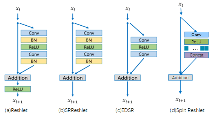
He et al. [11] introduce deep residual learning theory to solve the performance degradation problem in ResNet caused by the deepening of neural network layers. SRResNet [12] is the first method to apply residual learning to SISR. It extracts reconstruction features of HR images by residual learning blocks and restores high-quality HR images. Enhanced deep super-resolution network (EDSR) [13] also uses residual learning, but compared with ResNet and SRResNet, it proposes many improvements such as removing batch normalization (BN). Fig. 1 shows the three different modules using residual learning: the original ResNet [14], SRResNet, and EDSR networks, and we compare them. The original structure of residual learning is shown in Fig. 1(a), which was proposed by He et al. [11]. Fig. 1(b) shows SRResNet. We can find that it completely applies the residual learning of ResNet in the feature extraction module of image reconstruction.
In Fig. 1(c), the EDSR removes the BN layer from the network, because Nah et al. [15] argue that the BN layer normalizes the features and eliminates the range flexibility of the network. Importantly, they also show experimentally that this simple modification greatly improved the performance.
Fig. 1.
2.2 Depthwise Separable Convolution
Depthwise separable convolution is proposed by MobileNet [17], and it is a form of factorized convolution that factorizes standard convolution into depthwise convolution and pointwise convolution. Depthwise convolution can be regarded as group convolution, and pointwise is a way to maintain the flow of information between group convolutions. In Fig. 2, we can see the detailed calculation process about depthwise separable convolution. However, the size of depthwise group is different from other methods, in which the size of the group is equal to the size of the input channel. It indicates that each input channel has a corresponding convolution kernel for computation, which will reduce a large number of parameters and computation. Assuming that the input and output channels are 64, then we know that depthwise separable convolution computes 63 times fewer parameters than the original convolution. We
Fig. 2.
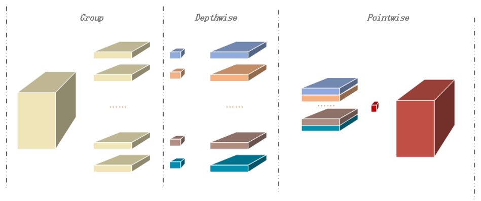
do not calculate the parameters of pointwise convolution, because the pointwise is an operation of 1×1 convolution, and its parameters are negligible compared with the general convolution. In conclusion, depthwise separable convolution is indeed a good way to reduce the computation and parameters of the networks.
3. Proposed Method
3.1 Model Design Analysis
From Fig. 3(a) and 3(b), we find that the super-resolution neural network mainly consists of a feature extraction network and an upsampling network. The feature extraction network mainly extracts the deep feature information required for image reconstruction from the original image, while the upsampling network uses deep feature information to reconstruct HR images. The upsampling strategy is less and fixed, so it is important to improve the image reconstruction quality by designing an efficient feature extraction network. From SRCNN [1] to wide activation super-resolution (WDSR) [18] and super-resolution feedback network (SRFBN) [19], they have been committed to changing the feature extraction network to improve the image super-resolution. Although the network goes from three to hundreds of layers, the quality of reconstructed images improved less in terms of PSNR (peak signal-to-noise ratio) [20] and SSIM (structural similarity index measure) [21]. The PSNR/SSIM of SRCNN is 30.48/0.8628 on the test ×4 Set5 image, while the PSNR/SSIM of SRFBN is 32.56/0.8992 on the test ×4 Set5 image. The depth of the feature extraction network increased hundreds of times, while PSNR and SSIM improved by 2.08 dB and 0.0364, respectively. In addition, SISR is a pixel-level task and relies on shallow pixel-level information during the construction process. Therefore, researchers should pay more attention to the pixel-level information at the shallow layer of the image when designing lightweight image super-resolution networks.
Fig. 3.
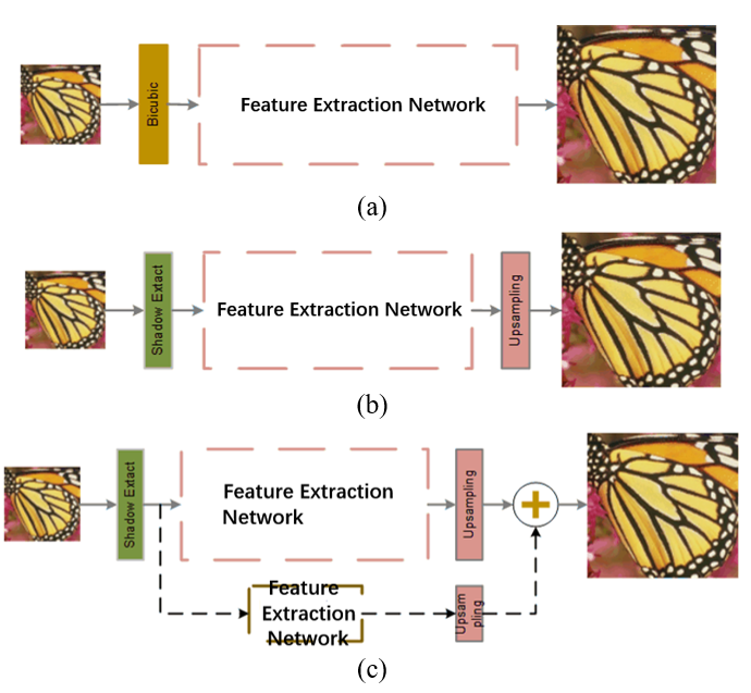
Table 1.
| [TeX:] $$32 \times \mathrm{C} \mathbf{c t} / \mathrm{ms}$$ | [TeX:] $$64 \times C \text { ct/ms }$$ | [TeX:] $$128 \times \mathrm{C} \mathrm{ct} / \mathrm{ms}$$ | |
|---|---|---|---|
| [TeX:] $$3 \times 3 \text { conv }$$ | 0.090 | 0.271 | 1.105 |
| ReLU | 0.034 | 0.066 | 0.131 |
| Sigmoid | 0.036 | 0.070 | 0.139 |
| Bias_add/add | 0.032 | 0.067 | 0.141 |
| concat | 0.041 | 0.042 | 0.045 |
| mul | 0.049 | 0.095 | 0.188 |
“C” represents the channel and “ct” represents the computation time cost.
Before designing a compact and lightweight network, we conducted experiments on the time cost of the fundamental operation of a convolutional neural network. These experiments use the TensorFlow framework and the TensorFlow Timeline tool to calculate time cost. All computation times in Table 1 are in milliseconds. From Table 1, we find that convolution is the most time-consuming compared with other operations. When the number of feature channels in the convolution layer is reduced by 1/2, the computation time of the convolutional layer is reduced by 3/4. But in other operations, the time reduction is not so strong. Therefore, reducing the number of convolutional channels and convolution operations is more beneficial to reducing the parameters and computation of the lightweight network.
3.2 Channel Split Residual
Through the experiments and analyses in Section 3.1, we can find that reducing the number of convolutional channels plays an important role in the lightweight of the whole network, so we propose the structure of channel split residual learning to reduce the number of convolutional channels. In the channel split residual learning (Fig. 1(d)), we combine the general residual learning method with the recently popular group convolution, and we retain the method proposed by EDSR [13] which removed the BN layer. Meanwhile, we adopt group convolution in the second convolution, where the number of groups is equal to the number of input channels. If the number of input channels is 64 and the number of output channels is the same as the number of input channels, the number of parameters of the residual module in EDSR [13] is [TeX:] $$3 \times 3 \times 64 \times 2$$ 2 (shown in Fig. 1(c)) and the number of parameters of the channel split residual structure is [TeX:] $$3 \times 3 \times 64 \times 64+3 \times 3 \times 1 \times 64+1 \times 1 \times 64$$ (shown in Fig. 1(d)), which reduces the parameters to 50.78%. Assuming the size of the input feature map is H×W, the number of the floating point of operations (FLOPs) of the residual module in EDSR is calculated as 50.82% of the original.
If the input and output feature maps are represented by [TeX:] $$X_{i} \text { and } X_{i+1},$$ respectively, the residual structure proposed by EDSR can be expressed by the formula (1):
(1)
[TeX:] $$X_{i+1}=f_{c o n v}\left(\operatorname{Re} L U\left(f_{c o n v}\left(X_{i}\right)\right)\right)+X_{i}$$Then the channel split residual structure can be described by the formula (2):
(2)
[TeX:] $$X_{i+1}=f_{G_{-} c o n n}\left(\operatorname{Re} L U\left(f_{c a n}\left(X_{i}\right)\right)\right)+X_{i}$$where ReLU represents the activation function and [TeX:] $$f_{\text {conv }}$$ is an ordinary convolution operation with a [TeX:] $$3 \times 3$$ kernel. [TeX:] $$f_{G_{-} \operatorname{conv}}$$ denotes the group convolution operation, G is the number of groups. In CSRNet, G is equal to the number of input channels. To maintain the data flow between the channels, we refer to the ordinary addition operation in the network. Compared with channel shuffling [22] and identity skipping method in Ghost module [23], our method is more straightforward and computationally convenient without adding additional computations, which is an advantage of general residual learning.
3.3 Double-Upsampling Network
There are two common types of upsampling networks: subpixel convolution and deconvolution. Subpixel convolution, proposed by ESPCN [2], is a method that corresponds the feature map to the HR image, which reduces the computation and memory consumption of deconvolution. In the subpixel, the extraction of HR features is the key to the quality of the reconstructed image since the final value of the HR feature map corresponds to the reconstructed HR image pixels one by one. It is different from other high-level visual tasks, which have far fewer prediction points than SISR. To reduce the pressure of feature extraction in the networks, we adopt a double-upsampling network structure, which is supplemented by a simple upsampling network compared with the general upsampling network. In Fig. 3(c), the depth feature extraction network in the red box is regarded as the residual network, marked as Res_Net, and the shadow network is regarded as the main network structure, marked as Main_Net. If [TeX:] $$X_{\text {input }}$$ is input as an LR image, [TeX:] $$Y_{r e}$$ as the reconstructed HR image, and the real HR image is [TeX:] $$Y_{H},$$ then the feature map [TeX:] $$X_{\text {res_map }}$$ extracted by Res_Net during the HR image reconstruction can be represented as:
The Main_Net feature map [TeX:] $$X_{\text {main_map }}$$ is represented as:
where [TeX:] $$f_{e x_{-} \text {res }} \text { and } f_{e x_{-} \text {main }}$$ represent the Res_Net feature extraction network and Main_Net feature extraction network, respectively, and the neural network structure is composed of multiple channels separated by residual structures. The whole reconstruction process is represented as:
(5)
[TeX:] $$Y_{r e}=f_{r E_{-} u p}\left(X_{r e S_{-} m q u}\right)+f_{m a n_{-} u p}\left(X_{m a n_{-} m a p}\right)$$where [TeX:] $$f_{\text {res_up }} \text { and } f_{\text {main_up }}$$ represent the upsampling network of Res_Net and Main_Net reconstructed networks, respectively, and the upsampling network adopts the subpixel convolution method.
In order to make the network easy to train, we propose a loss function for the double upsampling network. It is described as follows:
From the formula (6), we can find that the loss function of the double upsampling network consists of two components: [TeX:] $$\operatorname{loss}_{s} \text { and } \operatorname{los}_{o} \cdot \operatorname{loss}_{s}$$ represents the loss between the HR image reconstructed by Main_Net and the real HR image [TeX:] $$Y_{H}, \text { and } \operatorname{loss}_{o}$$ represents the loss between the final reconstructed HR image [TeX:] $$Y_{r e}$$ and the real HR image [TeX:] $$Y_{H}.$$ . To reduce the difference between the reconstructed HR image and the real image in Main_Net, the reconstruction loss of Main_Net is also added to the final loss, which can also reduce the learning pressure of the residual learning upsampling network.
3.4 Frame Rate Evaluation
The existing evaluation metrics for lightweight networks include the number of parameters and FLOPs, both of which are objective evaluation metrics. However, the inference speed of the neural network is expressed by this evaluation metric inaccurately due to the optimization of the GPU internal acceleration mechanism. The reduced parameters and the percentage of computation cannot be matched with the percentage increase of the actual computation speed. In Table 2, we perform three sets of comparison experiments in terms of convention structure, number of convolutional channels, and network depth. 10_res_block_64_ [TeX:] $$3 \times 3$$ is our baseline control group. Res_block represents residual blocks, 10 stands for the number of residual blocks, 64 stands for the number of convolutional channels, and [TeX:] $$3 \times 3$$ represents the size of the convolutional kernel. 10_res_block_64_ indicates that [TeX:] $$3 \times 1+1 \times 3$$ indicates that [TeX:] $$3 \times 3$$ convolution is replaced by the [TeX:] $$3 \times 1 \text { and } 1 \times 3$$ convolution. In Table 2, each experiment is tested three times on TITAN X GPU using the TensorFlow framework for an image size of [TeX:] $$256 \times 256.$$ . From Table 2, you can find that:
Compared with [TeX:] $$3 \times 3$$ convolution, [TeX:] $$3 \times 1 \text { and } 1 \times 3$$ convolutional groups require more computation time. In compact network design, replacing [TeX:] $$3 \times 3$$ convolution with [TeX:] $$3 \times 1 \text { and } 1 \times 3$$ convolutional groups does not reduce the computation time.
Theoretically, if the depth of the network is 1/2 of the original network, the time should be 1/2 of the original network, but in the experiment, the time is 4/7 of the original network.
Theoretically, if the number of channels of the network is 1/2 of the original network, and the time should be 1/4 of the original network, but in the experiment, the time is 1/3 of the original network.
The change of the number of channels has the greatest influence on the change of the whole network time, while the change of the convolutional kernel size has little influence on the change of the whole network time.
Table 2.
| test1 | test2 | test3 | ||||
|---|---|---|---|---|---|---|
| Frame rate | FPS (s) | Frame rate | FPS (s) | Frame rate | FPS (s) | |
| 10_res_block_64_[TeX:] $$3 \times 3$$ | 68.50 | 1.3800 | 69.83 | 1.4300 | 69.94 | 1.4300 |
| 10_res_block_64_[TeX:] $$3 \times 11 \times 3$$ | 60.23 | 1.6600 | 64.97 | 1.5300 | 59.18 | 1.6800 |
| 5_res_block_64_[TeX:] $$3 \times 3$$ | 116.31 | 0.8126 | 110.56 | 0.8635 | 117.88 | 0.8030 |
| 10_res_block_128_[TeX:] $$3 \times 3$$ | 29.00 | 3.3500 | 28.99 | 3.6632 | 28.58 | 3.6799 |
Therefore, we propose a new method to test the speed, but it requires a basic model as a baseline. As shown in Table 2, our baseline is 10_res_block_64_ [TeX:] $$3 \times 3.$$ The time cost of the test includes only the time of the feature extraction network. To minimize the bias in statistical computation, we performed three tests for each experiment. In the tests, we computed the time cost of 105 frames, but not 100 frames, which is described as T_100_frame. The computation time for the first 5 frames is unstable in TensorFlow because the GPU needs some more time to prepare at the beginning of the computation. The frame rate T_100_frame is as follows:
4. Experiments
4.1 Datasets and Metrics
In our experiments, we used the dataset DIV2K [24] to train the model, which contains 800 high-quality training images. First, we randomly cropped [TeX:] $$256 \times 256$$ images as the HR images and then generate the LR images with different down-sampling multiples from the HR images by bicubic interpolation. To increase the amount of training data, several dataset enhancement operations were performed on these images, including such as random level, flips, and rotation. We tested on four datasets, Set5 [25], Set14 [26], BSD100 [27], and Urban100 [28]. Set5 and Set14 are generally test benchmarks. BSD100 is composed of nature images from the segmentation dataset proposed by Berkeley Lab. Recently, the urban images provided by Huang et al. [28] are very interesting, because they contain many challenging images that are not available with existing methods. These four datasets can verify the effectiveness of the model. For the evaluation metric, two evaluation metrics are used: a measure of image quality and a lightweight network evaluation metric. The evaluation metrics for image quality include calculated PSNR and SSIM. The evaluation metrics for lightweight networks include parameters, Multi_Add, our proposed frame rate of 100 frames (100_FPS).
4.2 Implementation Details
In our network, the convolution kernels are set to [TeX:] $$3 \times 3.$$ The padding size of the convolution kernels is set to 1 to keep the size of the input and output feature maps consistent with the real HR images. The Res_Net uses a residual structure with 10 channel split residual blocks. In Res_Net, the first convolution uses [TeX:] $$643 \times 3 \times 64$$ convolution kernels, and the second convolution structure uses [TeX:] $$643 \times 3 \times 1$$ convolution kernels. In Main_Net, we only use a 5-layer general convolution as the feature extraction network. In Main_Net and Res_Net, we use the subpixel approach to generate high-resolution images. In training, we use the Adam optimizer [29] to minimize the loss function [TeX:] $$\operatorname{loss}_{a l l}.$$ The initial training sets the learning rate at 0.001, which decreases by a factor of 10 after [TeX:] $$3 \times 10^{4}$$ iterations. We implemented the proposed network using the PyTorch framework and trained it using an NVIDIA Titan X GPU. The entire model was trained in less than 1 day.
4.3 Ablation Analysis
To verify the validity of each part the proposed method, we conducted three groups of comparison experiments. In the ablation experiment, the baseline model is a residual learning structure proposed in EDSR. As can be found from Table 3, 10_res_block is the baseline model, and 10_res_split is our proposed channel splitting residual. Compared the first row with the second row, we can find that the parameters of the channel split residual are reduced by about 50% compared with the residual structure of EDSR. And the Multi_Adds of the channel split residual are reduced by about 75%. The amount of parameters and computations is reduced by about double and the frame rate is increased by 90%. The large reduction in parameters and computations also introduces some quality loss to the reconstructed images. In addition to testing the performance of the channel split residual structure, we also tested the performance of the double-upsampling network. The 10_res_split and 10_res_split_double in the table are used as a comparison experimental group. “Double” represents the double-upsampling network structure, and the unmarked one is the single upsampling network. From the two pairs of experiments, it can be found that the double-upsampling network has fewer parameters than the single-upsampling network in simple Res_Net, but the PSNR and SSIM are improved by 0.08 dB and 0.097, respectively. In terms of speed, the double-upsampling network does not increase the running time. Before the deep feature extraction network is finished in Res_Net, the shallow feature extraction network Main_Net has finished running and was waiting for the results of Res_Net. We also compared the loss function proposed for double-upsampling. 10_res_split_double_Lall indicates the use of a loss function [TeX:] $$\operatorname{loss}_{a l l},$$ 10_res_split_double indicates the use of loss function [TeX:] $$\operatorname{loss}_{o}.$$ Comparing this group of experiments reveals that the loss function [TeX:] $$\operatorname{loss}_{a l l}$$ contributes to improving the quality of the reconstructed images in the same structured network.
Table 3.
| set5_psnr | set5_ssim | Parameters | Multi_Adds | 100_FPS | |
|---|---|---|---|---|---|
| 10_res_block | 32.50 | 0.8973 | 2622k | 4292.5G | 62 fps |
| 10_res_split | 32.21 | 0.8577 | 1277k | 929.3G | 118 fps |
| 10_res_split_double | 32.29 | 0.8674 | 1297k | 1092.5G | 118 fps |
| 10_res_split_double_Lall | 32.34 | 0.8792 | 1297k | 1092.5G | 118 fps |
10_res_block is the feature extraction network consisting of 10 residual blocks in Fig. 1(c); “split” stands for the structure of channel split residual in Fig. 1(d); “double” represents the structure of the double-upsampling network in Fig. 3(c). “Lall” indicates that our proposed loss function for the double upsampling network.
In Table 4, the proposed method CSRNet is compared with some general SISR methods, such as SRCNN [1], DRRN [5], and EDSR [13], as well as with lightweight image super-resolution methods. Table 4 shows PSNR and SSIM for all methods tested on the three datasets. In contrast to the earlier lightweight network DRRN [5], which is a network with only 22 layers, the proposed method CSRNet has 40 layers. Therefore, the CSRNet has more parameters compared to DRRN. When we test on Set5, the CSRNet has 0.46 dB and 0.005 more than DRRN in PSNR and SSIM, respectively. Meanwhile, the CSRNet is slightly faster than DRRN in terms of computational speed. We also compared it with EDSR, which the proposed channel split residual learnings references. The number of parameters and computation of the CSRNet is about 50% of that of EDSR, and there are some significant improvements in frame rate with little loss in reconstruction. In Table 4, we also compare with the lightweight image super-resolution network of FALSR [9], IDN [7], and CARN [30]. These three methods are similar in parameters and calculation, but IDN performs better than the other two methods in the quality of reconstructed images. Compared with the other two methods, the PSNR and SSIM of our method are improved by about 0.2 dB and 0.02, respectively. Although the CSRNet is slightly more parametric and computationally intensive than CARN, and the computational speed is naturally inferior to it, the CSRNet has 0.42 dB more in PSNR than CARN. Compared with the latest method MADNet [31], the proposed CSRNet is inferior to MADNet in some evaluation metrics. It indicates that it is still room for improvement, and we will continue to work hard on lightweight SISR. By comparing the frame rate and PSNR together (Fig. 4), it can be seen that although the CSRNet is inferior to EDSR in performance, it is much faster than EDSR in speed. Our method is not as fast as AWSR [32], FALSR, and CARN in terms of speed, but far superior to these three methods in terms of performance.
Table 4.
| Scale | Methods | Parameters | Mult_Adds | 100_FPS | Set5 | Set14 | BSD100 |
|---|---|---|---|---|---|---|---|
| 2 | SRCNN [1] | 57k | 52.47G | 213 fps | 36.66/0.9542 | 32.42/0.9603 | 31.36/0.8879 |
| DRRN [5] | 297k | 6796.9G | 30 fps | 37.74/0.9591 | 33.23/0.9136 | 32.05/0.8973 | |
| EDSR [13] | 2662k | 4292.5G | 32 fps | 37.78/0.9597 | 32.28/0.9142 | 32.05/0.8973 | |
| AWSR [32] | 1397k | 320.5G | 56 fps | 38.11/0.9608 | 33.78/0.9189 | 32.49/0.9316 | |
| FALSR [9] | 326k | 74.7G | 76 fps | 37.82/0.9590 | 33.55/0.9168 | 32.10/0.8987 | |
| CARN [30] | 412k | 46.1G | 74 fps | 37.53/0.9583 | 33.26/0.9141 | 31.92/0.8960 | |
| IDN [7] | 590k | 81.87G | 64 fps | 37.83/0.9600 | 33.30/0.9148 | 32.08/0.8985 | |
| MADNet [31] | 1002k | 51.4G | 61 fps | 37.85/0.9600 | 33.38/0.9161 | 32.04/0.8979 | |
| Ours | 1297k | 1092.5G | 60 fps | 37.80/0.9600 | 32.29/0.9138 | 32.07/0.8976 | |
| 3 | SRCNN [1] | 57k | 52.47G | 213 fps | 32.75/0.9090 | 29.28/0.8209 | 28.41/0.7863 |
| DRRN [5] | 297k | 6796.9G | 30 fps | 34.03/0.9244 | 29.96/0.8347 | 28.95/0.8004 | |
| EDSR [13] | 2662k | 4292.5G | 32 fps | 34.09/0.9248 | 30.00/0.8350 | 28.96/0.8001 | |
| AWSR [32] | 1476k | 150.6G | 56 fps | 34.52/0.9281 | 30.38/0.8426 | 29.16/0.8069 | |
| CARN [30] | 412k | 46.1G | 74 fps | 33.99/0.9236 | 30.08/0.8367 | 28.91/0.8000 | |
| IDN [7] | 590k | 81.87G | 64 fps | 34.11/0.9253 | 29.99/0.8354 | 28.95/0.8013 | |
| MADNet [31] | 1002k | 51.4G | 61 fps | 34.16/0.9253 | 30.21/0.8398 | 28.98/0.8323 | |
| Ours | 1297k | 1092.5G | 60 fps | 34.10/0.9223 | 30.00/0.8332 | 28.97/0.8007 | |
| 4 | SRCNN [1] | 57k | 52.47G | 213 fps | 30.48/0.8628 | 27.49/0.7503 | 24.52/0.7221 |
| DRRN [5] | 297k | 6796.9G | 30 fps | 31.68/0.8888 | 28.31/0.7720 | 27.38/0.7284 | |
| EDSR [13] | 2662k | 4292.5G | 32 fps | 32.50/0.8973 | 28.72/0.7851 | 27.72/0.7418 | |
| AWSR [32] | 1587k | 91.1G | 56 fps | 32.27/0.8960 | 28.69/0.7843 | 27.63/0.7385 | |
| CARN [30] | 412k | 46.1G | 74 fps | 31.92/0.8903 | 28.42/0.7762 | 25.62/0.7694 | |
| IDN [7] | 590k | 81.87G | 64 fps | 31.82/0.8903 | 28.25/0.7730 | 27.42/0.7297 | |
| MADNet [31] | 1002k | 51.4G | 61 fps | 31.95/0.8917 | 28.42/0.7762 | 27.44/0.7327 | |
| Ours | 1297k | 1092.5G | 60 fps | 32.34/0.8674 | 28.49/0.7872 | 27.50/0.7399 |
The horizontal represents the evaluation metrics and datasets, and the vertical represents the current methods of image super-resolution using lightweight concepts. The results in the table are ×2 ×3 ×4 on Set5, Set14, and BSD100.
Fig. 4.
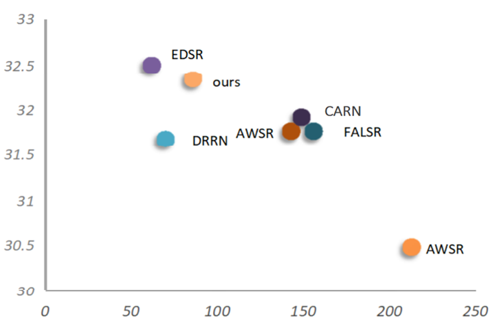
Fig. 5.
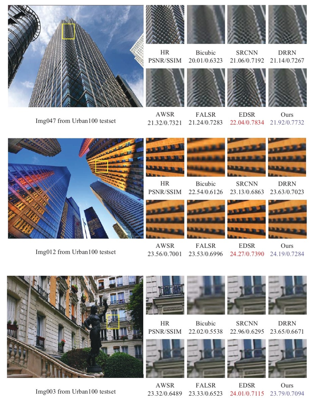
In addition, the CSRNet outperforms these methods in terms of performance and speed compared to the earlier DRRN methods. During the test, we selected three test images from Urban100 shown in Fig. 5. The image on the left is the original image, and the image on the right is the resulting image cropped from the yellow box. From the result images, we find that the reconstructed images of EDSR have the best visual effect, followed by ours. However, the reconstructed images of CSRNet look a little bit sharper compared to other lightweight methods. The CSRNet method has advantages and disadvantages com¬pared to the currently popular methods, but it is an effective and useable method.
5. Conclusion
The SISR research serves as a preprocessing work for many high-level visual tasks, which have a greater requirement for the inference speed of reconstructed HR images. Therefore, we introduce the idea of lightweight artificial design networks into this research direction of image super-resolution. To design the lightweight image super-resolution model, we propose the structures of channel split residual learning and double-upsampling. Channel split residual learning mainly uses group convolution to reduce the number of convolutional computation parameters and speed up the computation. Double-upsampling uses a two upsampling structure to widen the up-sampling network to ensure the performance of the lightweight network without adding extra computation time overhead. We demonstrate the effectiveness of our method on different datasets and find that our method is comparable to the state-of-the-art in terms of the quality of the reconstructed images. Making the network lighter and higher quality will be the work of the future.
Biography
References
- 1 C. Dong, C. C. Loy, K. He, X. Tang, in Computer Vision – ECCV 2014, Switzerland: Springer, Cham, pp. 184-199, 2014.custom:[[[-]]]
- 2 W. Shi, J. Caballero, F. Huszar, J. Totz, A. P. Aitken, R. Bishop, D. Rueckert, Z. Wang, "Real-time single image and video super-resolution using an efficient sub-pixel convolutional neural network," in Proceedings of the IEEE Conference on Computer Vision and Pattern Recognition, Las V egas, NV, 2016;pp. 1874-1883. custom:[[[-]]]
- 3 C. Dong, C. C. Loy, X. Tang, in Computer Vision – ECCV 2016, Switzerland: Springer, Cham, pp. 391-407, 2016.custom:[[[-]]]
- 4 J. Kim, J. K. Lee, K. M. Lee, "Deeply-recursive convolutional network for image super-resolution," in Proceedings of the IEEE Conference on Computer Vision and Pattern Recognition, Las V egas, NV, 2016;pp. 1637-1645. custom:[[[-]]]
- 5 Y. Tai, J. Yang, X. Liu, "Image super-resolution via deep recursive residual network," in Proceedings of the IEEE Conference on Computer Vision and Pattern Recognition, Honolulu, HI, 2017;pp. 2709-2798. custom:[[[-]]]
- 6 N. Ahn, B. Kang, K. A. Sohn, in Proceedings of the European Conference on Computer Vision (ECCV), Munich, Germany, 2018, pp, 256-272, 256-272. custom:[[[-]]]
- 7 Z. Hui, X. Wang, X. Gao, "Fast and accurate single image super-resolution via information distillation network," in Proceedings of the IEEE Conference on Computer Vision and Pattern Recognition, Salt Lake City, UT, 2018;pp. 723-731. custom:[[[-]]]
- 8 X. Chu, B. Zhang, R. Xu, H. Ma, 2019 (Online), Available: https://arxiv.org/abs/.01074, Available: https://arxiv.org/abs/1901.01074, 1901.custom:[[[-]]]
- 9 X. Chu, B. Zhang, H. Ma, R. Xu, Q. Li, "Fast, accurate and lightweight super-resolution with neural architecture search," in 2019 (Online). Available: https://arxiv.org/abs/1901.07261, 2019 (Online). Available: https://arxiv.org/abs/.07261, 1901;custom:[[[-]]]
- 10 B. Zoph, V. V asudevan, J. Shlens, Q. V. Le, "Learning transferable architectures for scalable image recognition," in Proceedings of the IEEE Conference on Computer Vision and Pattern Recognition, Salt Lake City, UT, 2018;pp. 8697-8710. custom:[[[-]]]
- 11 K. He, X. Zhang, S. Ren, J. Sun, "Deep residual learning for image recognition," in Proceedings of the IEEE Conference on Computer Vision and Pattern Recognition, Las V egas, NV, 2016;pp. 770-778. custom:[[[-]]]
- 12 C. Ledig, L. Theis, F. Huszar, J. Caballero, A. Cunningham, A. Acosta, et al., "Photo-realistic single image super-resolution using a generative adversarial network," in Proceedings of the IEEE Conference on Computer Vision and Pattern Recognition, Honolulu, HI, 2017;pp. 105-114. custom:[[[-]]]
- 13 B. Lim, S. Son, H. Kim, S. Nah, K. M. Lee, "Enhanced deep residual networks for single image super-resolution," in Proceedings of the IEEE Conference on Computer Vision and Pattern Recognition Workshops, Honolulu, HI, 2017;pp. 1132-1140. custom:[[[-]]]
- 14 Y. Zhang, K. Li, K. Li, L. Wang, B. Zhong, Y. Fu, in Proceedings of the European Conference on Computer Vision (ECCV), Munich, Germany, 2018, pp, 294-310, 294-310. custom:[[[-]]]
- 15 S. Nah, T. H. Kim, K. M. Lee, "Deep multi-scale convolutional neural network for dynamic scene deblurring," in Proceedings of the IEEE Conference on Computer Vision and Pattern Recognition, Honolulu, HI, 2017;pp. 257-265. custom:[[[-]]]
- 16 A. G. Howard, M. Zhu, B. Chen, D. Kalenichenko, W. Wang, T. Weyand, M. Andreetto, and H. Adam, 2017 (Online). Available:, https://arxiv.org/abs/1704.04861
- 17 B. Lim, S. Son, H. Kim, S. Nah, K. Mu Lee, "Enhanced deep residual networks for single image super-resolution," in Proceedings of the IEEE Conference on Computer Vision and Pattern Recognition Workshops, Honolulu, HI, 2017;pp. 1132-1140. custom:[[[-]]]
- 18 Z. Li, J. Yang, Z. Liu, X. Yang, G. Jeon, W. Wu, "Feedback network for image super-resolution," in Proceedings of the IEEE/CVF Conference on Computer Vision and Pattern Recognition, Long Beach, CA, 2019;pp. 3867-3876. custom:[[[-]]]
- 19 Z. Li, J. Yang, Z. Liu, X. Yang, G. Jeon, W. Wu, "Feedback network for image super-resolution," in Proceedings of the IEEE Conference on Computer Vision and Pattern Recognition, Long Beach, CA, 2019;pp. 3867-3876. custom:[[[-]]]
- 20 Z. Wang, A. C. Bovik, H. R. Sheikh, E. P. Simoncelli, "Image quality assessment: from error visibility to structural similarity," IEEE Transactions on Image Processing, vol. 13, no. 4, pp. 600-612, 2004.doi:[[[10.1109/TIP.2003.819861]]]
- 21 X. Zhang, X. Zhou, M. Lin, J. Sun, "Shufflenet: an extremely efficient convolutional neural network for mobile devices," in Proceedings of the IEEE Conference on Computer Vision and Pattern Recognition, Salt Lake City, UT, 2018;pp. 6848-6856. custom:[[[-]]]
- 22 K. Han, Y. Wang, Q. Tian, J. Guo, C. Xu, C. Xu, "Ghostnet: more features from cheap operations," in Proceedings of the IEEE/CVF Conference on Computer Vision and Pattern Recognition, Seattle, W A, 2020;pp. 1577-1586. custom:[[[-]]]
- 23 E. Agustsson, R. Timofte, "Ntire 2017 challenge on single image super-resolution: dataset and study," in Proceedings of the IEEE Conference on Computer Vision and Pattern Recognition Workshops, Honolulu, HI, 2017;pp. 1122-1131. custom:[[[-]]]
- 24 M. Bevilacqua, A. Roumy, C. Guillemot, M. L. Alberi-Morel, "Low-complexity single-image super-resolution based on nonnegative neighbor embedding," in Proceedings of the British Machine Vision Conference (BMVC), Surrey, UK, 2012;pp. 1-10. custom:[[[-]]]
- 25 R. Zeyde, M. Elad, M. Protter, in Curves and Surfaces, Germany: Springer, Heidelberg, pp. 711-730, 2010.custom:[[[-]]]
- 26 D. Martin, C. Fowlkes, D. Tal, J. Malik, "A database of human segmented natural images and its application to evaluating segmentation algorithms and measuring ecological statistics," in Proceedings 8th IEEE International Conference on Computer Vision (ICCV), V ancouver, Canada, 2001;pp. 416-423. custom:[[[-]]]
- 27 J. B. Huang, A. Singh, N. Ahuja, "Single image super-resolution from transformed self-exemplars," in Proceedings of the IEEE Conference on Computer Vision and Pattern Recognition, Boston, MA, 2015;pp. 5197-5206. custom:[[[-]]]
- 28 D. P. Kingma and J. Ba, 2014 (Online). Available:, https://arxiv.org/abs/1412.6980
- 29 N. Ahn, B. Kang, K. A. Sohn, in Proceedings of the European Conference on Computer Vision (ECCV), Munich, Germany, 2018, pp, 256-272, 256-272. custom:[[[-]]]
- 30 Y. Zhang, Y. Tian, Y. Kong, B. Zhong, Y. Fu, "Residual dense network for image super-resolution," in Proceedings of the IEEE Conference on Computer Vision and Pattern Recognition, Salt Lake City, UT, 2018;pp. 2472-2481. custom:[[[-]]]
- 31 R. Lan, L. Sun, Z. Liu, H. Lu, C. Pang, X. Luo, "MADNet: a fast and lightweight network for single-image super resolution," IEEE Transactions on Cybernetics, vol. 51, no. 3, pp. 1443-1453, 2020.custom:[[[-]]]
- 32 L. Zhang, P. Wang, C. Shen, L. Liu, W. Wei, Y. Zhang, A. Van Den Hengel, "Adaptive importance learning for improving lightweight image super-resolution network," International Journal of Computer Vision, vol. 128, no. 2, pp. 479-499, 2020.custom:[[[-]]]