Aili Gao , Lan Chen , Xiaohan Wei , Chao Liu and Lihua Cheng
Spatial Distribution Prediction and Migration Characteristic of Petroleum Hydrocarbons in Soil Based on Artificial Neural Networks
Abstract: Soil pollution resulting from petroleum hydrocarbons (PHCs) arising from industrialization and human activities has emerged as a progressively severe global concern. Establishing an accurate spatial distribution prediction model for PHCs through limited sampling data play an important role in understanding the migration characteristics of PHCs and effectively preventing soil pollution. This article employs soil samples within 8 m of a chemical plant, in conjunction with hydrogeological data, to model the spatial distribution of PHC content using a feedforward neural network (FNN). The prediction outcomes are characterized through three-dimensional visualization. The findings indicate that FNN demonstrates superior estimation accuracy compared to traditional interpolation method. Regarding the horizontal distribution within surface soil, there is pronounced lateral migration of PHC content in both the storage area and manufacturing shop, with migration aligning following the direction of groundwater. Vertically, PHC content exhibits a consistent pattern of increasing and then decreasing with greater depth. It is predominantly enriched in the lower section of the aeration zone and the upper part of the saturated zone, particularly within 4 m, under influence of groundwater. In this study, the prediction model offers an original approach to the spatial distribution of soil pollutants.
Keywords: Feedforward Neural Networks , Migration Characteristics , Petroleum Hydrocarbon , Spatial Distribution
1. Introduction
Petroleum, as an energy source, fuel and chemical raw material, is widely used in industry, agriculture, transportation and daily life. With the continuous increasing availability of petroleum products, large quantities of petroleum hydrocarbons (PHCs) and its products enter the soil during the processing of petroleum. It is estimated that more than 5 million sites worldwide are potentially contaminated, with PHC contaminated sites accounting for about one-third of the total number of contaminated sites. Based on the available findings, in most provinces in China, PHCs are the top three characteristic contaminants detected in soil from construction sites.
PHCs are complex mixtures of substances, mainly including alkanes, cycloalkanes, olefins, aromatic hydrocarbons, etc., PHCs that enter the soil will damage the physicochemical properties of the soil, affect soil permeability, and reduce soil quality, as well as pose a threat to public health and ecological safety due to their high toxicity, difficulty in degradation, and carcinogenicity and mutagenicity [1,2]. PHC contamination has become a worldwide environmental problem. Understanding the spatial distribution and migration characteristics of PHCs in soil, in particular, the distribution of pollutants in the depth of the soil is essential for the effective prevention and management of soil pollution.
Field sampling is a dependable method for obtaining accurate pollutant concentrations in the deeper layers of soil. However, the sampling process is time-consuming, expensive, and constrained by the limited number of sampling sites, thereby substantially restricting our comprehension of the distribution of soil contamination. Spatial interpolation models can assess the spatial distribution of contaminant concentrations in the field environment using limited soil sample data. Utilizing these interpolation models, we can achieve spatial characterization of regional soil contaminants, thereby refining our assessment perspective to specific points or partial areas. Kriging interpolation is the most widespread interpolation method. Nevertheless, this method assumes homogeneity in the study area, resulting in a smoothing effect during interpolation. This smoothing effect could potentially lead to the loss of essential soil attribute information in anomaly areas or inaccuracies in the interpolation expression. Kriging falls short in characterizing the complexity, multidimensionality, and uncertainty inherent in soil systems. The artificial neural network is an intricately complex nonlinear dynamic system with robust self-adaptation, self-organization, and self-learning capabilities. It has the capacity to emulate various nonlinear mapping relationships. Compared with conventional spatial interpolation methods, artificial neural network was proved that is suitable to the three-dimensional (3D) spatial distribution of diverse and variable soil pollutants. Hence, employing artificial neural networks for predicting the spatial distribution of soil pollutants can yield scientifically sound assessment results.
This article utilizes soil samples within 8 m of a chemical plant, along with hydrogeological data, to model the spatial distribution of PHCs content. The prediction results are characterized by 3D visualization. From a visualization perspective, we delved deeply into the migration characteristics of PHCs in the soil. This study can make contributions to the pollution control of PHCs, as well as other pollutants.
The primary contributions can be summarized as follows:
& centerdot; Formulate a field sampling program, carry out on-site drilling to reveal the environmental hydrogeological conditions of the land parcels, obtain the physical and chemical characteristics of the soil in each layer, collect soil samples and determine PHCs content.
& centerdot; Application of feedforward neural network (FNN) to construct a spatial distribution model of PHCs, visualize the distribution of PHCs in the soil, realize 3D visualization of the distribution of pollutants, and then deeply analyze the characteristics of petroleum level and vertical migration.
2. Review of Related Studies
Scholars at home and abroad have carried out a large number of studies on the migration and transformation laws of petroleum compounds in soil. Early studies were dominated by indoor experiments, and a wealth of theoretical research results were accumulated through soil column experiments, centrifugal experiments and biodegradation experiments, etc. However, the research space was mainly focused on one-dimensional (1D) and two-dimensional (2D) planar bases. Soil is a 3D natural space entity, and in-plane characterization of pollutant migration and distribution is relatively one-sided and isolated, making it difficult to comprehensively and accurately reflect the hydrogeological situation of the subsurface environment, the spatial distribution of pollutants and diffusion trends. In recent years, soil pollution research has been expanded from 2D space to 3D space, and spatial interpolation models have been widely used for soil pollution distribution prediction, but each interpolation method has specific assumptions, such as deterministic interpolation models (e.g., inverse distance weighting) do not take into account spatial structural information and the correlation between spatial distribution calculation, and geostatistical methods (e.g., kriging interpolation) interpolation techniques have a smoothing effect, which may result in the underestimation of locally high values or the overestimation of locally low values, resulting in the bias in the assessment of soil contamination, and having an impact on related decision-making.
With the rapid development of computer technology, machine learning models have been widely used in various fields such as construction, medicine and health, in soil science the application of artificial neural networks in machine learning is receiving more and more attention [3-5]. Shi et al. [6] constructed a heavy metal content estimation model using surface soil sampling data, and compared the estimation accuracy of the spatial interpolation method with that of the machine learning model, and concluded that the machine learning model was more accurate. Zheng et al. [7] utilized bidirectional long short-term memory (Bi-LSTM) neural network to develop a spatial classification model for prediction of DEHP concentrations at different locations. Li et al. [8] found that artificial neural network is more accurate than linear regression prediction model, then used artificial neural network to evaluate cadmium contamination in farmland soils.
From the current research results and progress, artificial neural networks can effectively predict the spatial distribution of soil pollutants, and the prediction accuracy is higher than the previously commonly used spatial interpolation model, but the model prediction is mostly applied to the horizontal spatial distribution of surface soil pollutants, and there are fewer studies on the 3D spatial distribution. In this study, artificial neural networks were used to carry out the calculation of the 3D spatial distribution of PHCs in soil and the study of migration characteristics, and the results of the research can be visualized to understand the spatial distribution characteristics of PHCs, and better illustrate the spatial hierarchy of the stratum and the information of the 3D spatial distribution of PHCs.
3. Materials and Methods
3.1 Study Area
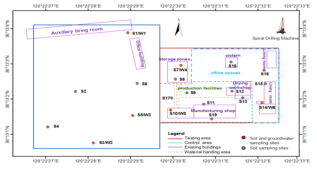
The study area is located in Qingdao, China (Fig. 1), covering an area of 11,600 m2, and is divided into two sections: control area and testing area. Initially, the control area functioned as an office space, the testing area housed a chemical company engaged in the production of methyl methacrylate-butadiene-styene (MBS) resins. The chemical company had a 15-year operational history and comprised production facilities, storage zones, and office spaces. All buildings and production facilities had been dismantled after 2022. Nineteen soil sampling sites, designated as S1 to S19, were established in the study area, with sampling depths ranging from 5.5 m to 8 m below the surface. Additionally, groundwater wells were installed in six of these sites. The monitoring factors of the samples are PHCs and pH. PHCs were analyzed by gas chromatography, pH was determined by potentiometric method.
3.2 Methods of Construction of Geologic Models
Interpolation and modeling of geologic data is essential to reconstruct the subsurface hydrogeologic structure of the study area and to gain insight into contaminant transport processes. In this research, we developed a site stratigraphic model using the 3D radial basis function interpolation method. This model is based on sampling point coordinates and core stratigraphic information.
The 3D radial basis function interpolation method first choose the appropriate radial basis function, commonly used radial basis function has a Gaussian surface function, polynomial function, linear function, etc. In this paper, Gaussian surface function is chosen, for each known data point, interpolation function in the point is equal to the value of the known data value, and then construct a system of linear equations to solve the interpolation function of the weight coefficients. For each data point, a linear equation can be constructed where the unknown is the weight coefficient. The weight coefficients of the interpolating function can be obtained by combining a system of linear equations for all data points and solving that system of linear equations. This is shown in the following equation:
where [TeX:] $$c_0, c_1, \lambda_i$$ are the weights, [TeX:] $$\varphi\left(\left|x-x_i\right|\right)$$ is the radial basis function, [TeX:] $$x_i$$ is the set of known data points.
3.3 Methods of Construction of Geologic Models
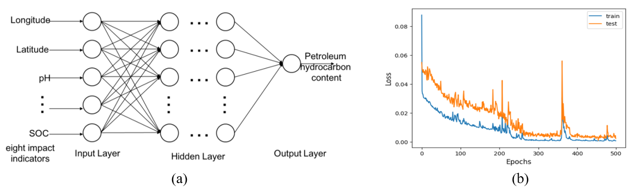
On the basis of site stratigraphic modeling, the results of soil borehole sample testing and analysis were combined with the borehole stratigraphic data to construct a PHC contamination distribution model based on the FNN, and at the same time, the Kriging interpolation method was introduced for the comparison of prediction accuracy. FNN is a classical model in artificial neural networks, and its structure includes input, hidden and output layers (Fig. 2(a)). For multi-layer artificial neural networks, the structure of neurons is similar to the structure of the human brain, with each neuron connected to other neurons by a specific coefficient [9]. This type of model is characterized by a computational process in which the input values are passed sequentially from the input layer to the hidden layer output layer, which ultimately produces the output.
Due to the limited field sampling data, a single use of all the data to train the model is likely to lead to overfitting, so the study uses a 10-fold cross-validation, the dataset will be divided into 10, each time to select 9 as the training set, the remaining 1 as the validation set, repeat the process for 10 times, each copy of the data have been used as a validation set, and have been used as a training set, there will not be a problem with the data to bring about the model bias, and at the same time, based on the evaluation of the results of the selection of hyper parameters. In this study, a total of eight influence indicators, including longitude, latitude, depth, pH, soil permeability coefficient, wet bulk density, organic carbon (OC) and specific yield, were used as the input part of the model, and the PHC content at the specified location was used as the output part, so the number of nodes in the input layer was eight and the number of nodes in the output layer was one, and the four implicit layers were chosen, whose nodes were 64, 32, 16, and 8, respectively. The data from each node is passed to a specific output function, called the activation function, which serves to nonlinearize the data, the ReLU function is applied to the implicit layer in the study, the ReLU function expression is shown in Eq. (2), each connection between two nodes represents a weighted value for the inputs to that connection, called weights, the weight values for each layer can be adjusted by training. The learning rate can determine the rate of change of the weights produced in each cycle, the study uses a fixed learning rate of 0.01, loss function uses the mean square error (MSE), whose expression is shown in Eq. (3), reflecting the difference between the predicted value and the true value, through repeated iterative operations, to determine the optimal number of learning iterations for the convergence of the value of the loss function (300 times) in Fig. 2(b) and the weights coefficient (3393), learning and training process is finished, and the model is established. The specific model parameters are shown in Table 1.
In this study, Python and TensorFlow were used to calculate the spatial distribution of PHCs, ArcGIS 10.8 was used to map the location of the study area and the distribution of the sampling points, Origin 2021 was used for mapping the statistical analysis of the sample data, and surf 25.1 was used for mapping the 3D spatial distribution of geology and PHC content.
4. Results and Discussion
4.1 Statistical Characteristic of Hydrogeology and PHC Content in the Study Area
The depth of the boreholes in the study area ranges from 5.5 m to 8 m. The investigation results show that the stratigraphic structure of the parcel is clear, and four parts of the soil layers are exposed (Fig. 3), the first layer of 0.7 m to 2.6 m thick is miscellaneous fill, the second layer of 0.7 m to 3.0 m thick is coarse sand, the third layer of 1.0 m to 4.6 m thick is silty sandy soil, and the fourth layer of 0.4 m to 1.0 m thick is powdery clay. During the investigation period, the shallow groundwater flowed from northeast to southwest, and the depth of the water table ranged from 1.10 m to 2.70 m. It was deposited in the miscellaneous fill, coarse sand and silty sandy soil. The transport of PHCs is affected by a variety of factors such as pH, porosity, OC, and other soil environmental conditions, soil properties, etc. [10]. According to the hydrogeological data of the study area, on-site stratigraphic drilling and experimental testing results, the relevant soil environmental conditions and physicochemical characteristics parameters of the study area are shown in Table 2.
Fig. 3.
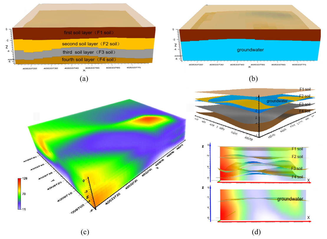
Table 2.
| Soil layer name | pH | Wet bulk density (g/cm3) | K (cm/s) | OC (g/kg) | Specific yield |
|---|---|---|---|---|---|
| First layer | 7.27–8.58 | 1.43 | 0.0087 | 0.83 | 0.14 |
| Second layer | 7.15–8.32 | 1.46 | 0.0174 | 0.41 | 0.27 |
| Third layer | 7.12–8.40 | 1.53 | 0.0116 | 0.36 | 0.26 |
| Fourth layer | 7.02–9.08 | 1.62 | 0.000023 | 0.17 | 0.02 |
A total of 95 soil samples and 6 groundwater samples were collected from the study area. The detection rate of PHC in 27 soil samples from the control area was 78%, all of the 68 soil samples from the testing area were detected with PHCs. The results indicated that PHCs were commonly present in the study area soil. The pH of the groundwater samples ranged from 7.16 to 7.51, and the PHCs were not detected.
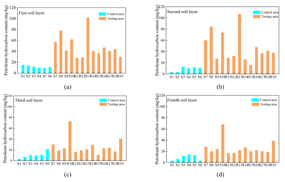
The control area was formerly an office area with no apparent source of PHC pollution. Therefore, the monitoring values were lower overall. The specific content varied from 10 to 15 mg/kg in the first layer, non-detected to 13 mg/kg in the second layer, non-detected to 21 mg/kg in the third layer, non-detected to 14 mg/kg in the fourth layer, and the mean values of the four layers were 12 mg/kg, 8.7 mg/kg, 10.1 mg/kg, and 8.5 mg/kg, respectively (Fig. 4). The testing area was a chemical company. The PHC content in the soil is higher than that in the control area, mainly originate from industrial activities in the neighborhood, including raw materials fueling use, automobile exhaust, etc. PHC content in the soil varied from 26 to 108 mg/kg in the first layer, 16 to 107 mg/kg in the second layer, 11 to 73 mg/kg in the third layer, and 17 to 68 mg/kg in the fourth layer, and the mean values of the four layers were 49.2 mg/kg, 48.2 mg/kg, 26.8 mg/kg, and 26.4 mg/kg, respectively. The content of PHCs in the testing area has some spatial discrete characteristics with medium discrete intensity.
Fig. 4.
4.2 Modeling the Spatial Distribution of PHCs
The above classical statistical analysis of PHC content summarizes the overall characteristics of soil PHC changes with depth, such as the control plot PHC content with depth increase overall change is not obvious, the experimental plots PHC content with depth increase shows an increase and then decrease in the trend, but does not reflect the PHC contamination characteristics of the different layers of the soil, the different production function areas, so the study based on feed-forward neural network to establish a PHC 3D spatial distribution model, in order to further analyze the spatial distribution of the content of PHCs in the soil, the migration law and the characteristics of the local changes in the region.
In view of the low distribution of PHC pollutant content in the control plots, this study focuses on the spatial distribution modeling of PHC pollution in the experimental plots. During the model construction process, ordinary kriging interpolation is used to compare the interpolation accuracy verification with FNN. The Gaussian model with the largest coefficient of determination and the smallest squared residuals was chosen after the normality test on the test data during ordinary kriging interpolation. Root mean square error (RMSE), coefficient of determination ([TeX:] $$R^2$$) and mean absolute error (MAE) were used as evaluation metrics for comparing the accuracy and precision of FNN with OK. The formulas are shown below:
(5)
[TeX:] $$R^2=1-\frac{\sum_{i=1}^n\left(y_i-\hat{y}\right)^2}{\sum_{i=1}^n\left(y_i-\bar{y}\right)^2},$$
where n denotes the number of samples, [TeX:] $$\hat{y}$$ is the predicted value of the sample, [TeX:] $$y_i$$ is the measured value, and [TeX:] $$\bar{y}$$ is the mean value.
Table 3.
| Method | Correlation coefficient (R2) & uparrow; | MAE (mg/kg) & downarrow; | RMSE & downarrow; |
|---|---|---|---|
| FNN | 0.971 (+0.020) | 4.248 (-0.566) | 5.402 (-1.689) |
| Ordinary Kriging | 0.951 (-) | 4.814 (-) | 7.091 (-) |
As Table 3 reveals, the FNN approach had smaller RMSE than kriging interpolation model (reduced by 1.689), and the comparative results show that the FNN predicts better.
The spatial distribution model of PHCs can be displayed in the 3D Viewer Window of Surfer and can be overlaid with the geologic model, as shown in Fig. 3.
4.3 Characterization of the Spatial Distribution of PHCs
The results of the 3D spatial distribution visualization in the study were sliced horizontally according to different soil layers. Superimposing the borehole points and plant plan to the distribution map of PHC content in the surface soil (Fig. 5(a)), the analysis showed that the highest concentration of PHCs was found at point S13, followed by points S12 and S8. This spatial distribution pattern is related to the original plant production layout, S13, S12, S8 points were distributed in the drying workshop diesel boiler room, drying tower, storage zones, diesel or raw material storage tanks and pipelines occurring in the phenomenon of “running, bubbling, dripping,” and so on, may be the main cause of PHC pollution. It was found that the farther away from the diesel boiler room the lower the concentration of PHCs in the surface layer, the farther away from the storage tanks on the west side of the storage tank area the concentration of PHCs gradually increased, and the farther away from the workshop on the southwestern side of the production workshop the concentration of PHCs also showed a trend of gradual increase. The concentration of PHCs in the surface layer of the storage tank area and production workshop shows obvious lateral migration, with the overall migration trend from northeast to southwest, mostly in the west, and in the same direction as the groundwater flow.
Fig. 5(b) PHC vertical distribution, and combined with the original plant layout and historical production activities analysis, PHC pollution is mainly concentrated in the drying workshop, storage tanks and production workshop, with the increase in depth, the PHC content are showing first increase and then reduce the law of change, of which the drying workshop, the tanks and the PHC concentration in the second layer reached the peak, corresponding to the depth of 2.6 m, 2.5 m, respectively. The concentration of PHCs in the production workshop peaked at about 5.0 m in the third layer.
The variability in the results of the study may be due to the fact that the sources of pollution in the production plant are mainly butadiene, styrene, and formaldehyde methyl acrylate, the sources of pollution in the storage tank area contain diesel fuel, etc., in addition to the above three types of substances, and the sources of pollution in the drying tower are mainly diesel fuel. Butadiene, styrene, and methyl formaldehyde acrylate, with carbon chains in the range of C4 to C8, are light-component substances with low molecular weights, exist mainly in the dissolved state, and are susceptible to lateral and vertical migration under the action of volatilization and groundwater transport. Diesel carbon chain in the range of C10–C22, belonging to the reorganization of the material, diesel viscosity is relatively large, viscous, easy to be retained to the surface layer and the subsurface layer of the Department, is not easy to lateral migration, but also not easy to migrate to the deeper layers.
Fig. 5.
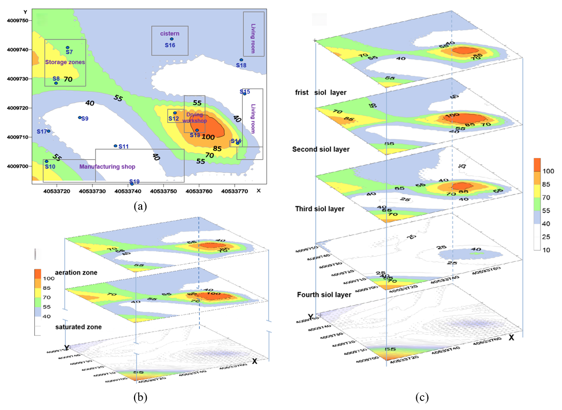
PHCs also showed uneven distribution characteristics in different soil layers. The content of PHCs in the first layer of miscellaneous fill increased gradually with depth, the concentration of PHCs in the second layer of coarse sand layer and the third layer of silty sand layer showed a gradual decrease in the rest of the area except for the southwest corner where the concentration of PHCs increased gradually with depth, and the PHCs content in the fourth layer of clay gradually decreased with the increase of depth. Relevant studies have shown that soil adsorption capacity is related to soil physicochemical characteristics, the weaker the infiltration capacity, the more conducive to the adsorption and retention of PHCs in the soil, and at the same time the adsorption capacity is directly proportional to the content of organic matter. Combined with the physical and chemical properties of the soil (Table 2), the soil layer with the largest adsorption capacity was the miscellaneous fill, followed by coarse sand, silty sand, and clay was the smallest, but the profiling in Fig. 5(b) showed that the largest PHCs content in each soil layer was the coarse sand, followed by the miscellaneous fill, silty sand, and clay. The permeability of coarse sand is stronger than that of miscellaneous fill, and the organic carbon content is lower than that of miscellaneous fill, but the overall PHCs are higher, which may be due to the fact that PHCs are affected by groundwater pressure at the same time during the migration process of each soil layer. Groundwater level and geologic structure map dissection (Fig. 4(d)) shows that the groundwater level is located in the vicinity of the boundary of the miscellaneous fill and coarse sand, and the miscellaneous fill is mainly located in the air-packed zone, where the vertical migration of PHCs is dominated and affected by the cumulative release factor. The coarse sand is in the water-saturated zone, and the distribution of PHCs in the soil layer at the groundwater surface (Fig. 5(c)) is roughly the same as that in the surface layer of the coarse sand, and the migration pattern of PHCs with groundwater in this soil layer changes, and PHCs are mostly enriched in the vicinity of the groundwater surface, i.e., at the surface of the coarse sand layer, and migrate with the groundwater through convection or diffusion.
5. Conclusion
In this paper, a spatial distribution prediction model of PHC contamination in soil was constructed based on FNN. Compared with the previous interpolation method, the prediction method is more accurate, and can more precisely reflect the overall contamination level of the site or the concentration level of vertical stratification under the limited sampling data. The study realizes 3D contamination inscription of real sites through spatial statistics and machine learning, which can overcome the shortcomings of the traditional single spatial statistical prediction model and reduce the cost of investigation at the same time. The results show that small molecular weight PHCs are more likely to migrate laterally and vertically than large molecular weight PHCs and the direction of lateral migration is the same as the direction of groundwater flow, while the vertical migration is affected by the pressure of groundwater at the same time, and is mostly enriched near the groundwater surface.
Since PHCs were not detected in the groundwater of the site, the study only discussed the spatial distribution and migration of PHCs in soil, and the study factors and scenarios were relatively simple, and the scope of the study will be further extended to conduct the modeling of the integrated pollution system under multi-scenario conditions in order to solve the site contamination problems under the complex water table geological environment. For the FNN model, the ablation of FNN inputs can be an option for future study.
Biography
Alli Gao
https://orcid.org/0009-0008-8321-9425
She received a B.S. degree in School of Civil Engineering at Jinan University in 2008, M.S. degree in School of Environmental and Municipal Engineering at Qingdao University of Technology in 2010. She is a senior engineer, now pursuing her Ph.D. in Environmental and Municipal Engineering at Qingdao University of Technology. Her research interests include wastewater treatment, resource utilization, soil pollution and risk assessment.
Biography
Lan Chen
https://orcid.org/0009-0002-9366-3809
She received B.S. degree in School of Petroleum and Environmental Engineering from Yan’an University in 2021. Since September 2022, she has been pursuing her M.S. degree in Environmental and Municipal Engineering at Qingdao University of Technology. Her current research interest is ecosystem analysis.
Biography
Xiaohan Wei
https://orcid.org/0009-0007-5269-1797
She received B.S. and M.S. degrees in School of Environmental and Municipal Engineering at Qingdao University of Technology in 2016 and 2019, respectively. She is now pursuing her Ph.D. in the same field from the same university. Her research interests include wastewater treatment, resource utilization, and electrochemical advanced oxidation technology.
Biography
Chao Liu
https://orcid.org/0009-0001-7842-9064
She received B.S. degree in School of Environmental Engineering from Inner Mongolia University of Technology in 2004. She received M.S. degrees and Ph.D. degree in School of Environmental and Municipal Engineering at Qingdao University of Technology in 2007 and 2018, respectively. She is currently an associate professor in School of Environmental and Municipal Engineering, Qingdao University of Technology in China. Her research interests include ecosystem analysis and optimized control of wastewater treatment plant operations.
Biography
Lihua Cheng
https://orcid.org/0000-0002-4806-5239
She received B.S. degree in School of Environmental and Municipal Engineering at Harbin University of Civil Engineering and Architecture in 1995. She received M.S. degree and Ph.D. degree in the same field from the same university in 1998 and 2001, respectively. She is a professor in the School of Environmental and Municipal Engineering at Qingdao University of Technology in China. Her research interests include technology for wastewater treatment and resource utilization, disinfection, and membrane contamination control.
References
- 1 D. Daassi and F. Qabil Almaghribi, "Petroleum-contaminated soil: environmental occurrence and remediation strategies," 3 Biotech, vol. 12, no. 6, article no. 139, 2022. https://doi.org/10.1007/s13205-022-03198-zdoi:[[[10.1007/s13205-022-03198-z]]]
- 2 A. A. Elijah, "A review of the petroleum hydrocarbons contamination of soil, water and air and the available remediation techniques, taking into consideration the sustainable development goals," Earthline Journal of Chemical Sciences, vol. 7, no. 1, pp. 97-113, 2022. https://doi.org/10.34198/ejcs.7122.97113doi:[[[10.34198/ejcs.7122.97113]]]
- 3 D. Zhao, Y . Liu, G. Zeng, X. Wang, S. Miao, and W. Gao, "A knowledge-based human-computer interaction system for the building design evaluation using artificial neural network," Human-Centric Computing and Information Sciences, vol. 13, article no. 2, 2023. https://doi.org/10.22967/HCIS.2023.13.002doi:[[[10.22967/HCIS.2023.13.002]]]
- 4 S. S. Alotaibi, H. A. Mengash, S. Dhahbi, S. Alazwari, R. Marzouk, M. A. Alkhonaini, A. Mohamed, and A. M. Hilal, "Quantum-enhanced machine learning algorithms for heart disease prediction," Human-Centric Computing and Information Sciences, vol. 13, article no. 41, 2023. https://doi.org/10.22967/HCIS.2023.13.041doi:[[[10.22967/HCIS.2023.13.041]]]
- 5 W. Ding, "Role of sensors based on machine learning health monitoring in athletes’ wearable heart rate monitoring," Human-Centric Computing and Information Sciences, vol. 13, article no. 16, 2023. https://doi.org/10.22967/HCIS.2023.13.016doi:[[[10.22967/HCIS.2023.13.016]]]
- 6 S. Shi, M. Hou, Z. Gu, C. Jiang, W. Zhang, M. Hou, C. Li, and Z. Xi, "Estimation of heavy metal content in soil based on machine learning models," Land, vol. 11, no. 7, article no. 1037, 2022. https://doi.org/10.3390/land11071037doi:[[[10.3390/land11071037]]]
- 7 S. Zheng, J. Wang, Y . Zhuo, D. Yang, and R. Liu, "Spatial distribution model of DEHP contamination categories in soil based on Bi-LSTM and sparse sampling," Ecotoxicology and Environmental Safety, vol. 229, article no. 113092, 2022. https://doi.org/10.1016/j.ecoenv.2021.113092doi:[[[10.1016/j.ecoenv.2021.113092]]]
- 8 C. Li, C. Zhang, T. Y u, X. Liu, Y . Yang, Q. Hou, Z. Yang, X. Ma, and L. Wang, "Use of artificial neural network to evaluate cadmium contamination in farmland soils in a karst area with naturally high background values," Environmental Pollution, vol. 304, article no. 119234, 2022. https://doi.org/10.1016/j.envpol.2022.119234doi:[[[10.1016/j.envpol.2022.119234]]]
- 9 M. M. Mijwel, "Artificial neural networks advantages and disadvantages," Mesopotamian Journal of Big Data, vol. 2021, pp. 29-31, 2021. https://doi.org/10.58496/MJBD/2021/006doi:[[[10.58496/MJBD/2021/006]]]
- 10 L. Wang, Y . Cheng, R. Naidu, and M. Bowman, "The key factors for the fate and transport of petroleum hydrocarbons in soil with related in/ex situ measurement methods: an overview," Frontiers in Environmental Science, vol. 9, article no. 756404, 2021. https://doi.org/10.3389/fenvs.2021.756404doi:[[[10.3389/fenvs.2021.756404]]]