Dingkang Hua , Qian Zhang , Wan Liao , Bin Wang and Tao Yan
CAttNet: A Compound Attention Network for Depth Estimation of Light Field Images
Abstract: Depth estimation is one of the most complicated and difficult problems to deal with in the light field. In this paper, a compound attention convolutional neural network (CAttNet) is proposed to extract depth maps from light field images. To make more effective use of the sub-aperture images (SAIs) of light field and reduce the redundancy in SAIs, we use a compound attention mechanism to weigh the channel and space of the feature map after extracting the primary features, so it can more efficiently select the required view and the important area within the view. We modified various layers of feature extraction to make it more efficient and useful to extract features without adding parameters. By exploring the characteristics of light field, we increased the network depth and optimized the network structure to reduce the adverse impact of this change. CAttNet can efficiently utilize different SAIs correlations and features to generate a high-quality light field depth map. The experimental results show that CAttNet has advantages in both accuracy and time.
Keywords: Attention Network , Deep Learning , Depth Estimation , Light Field
1. Introduction
In traditional photography, the camera forms pixel values by recording light rays in diverse directions, but this results in the loss of information about the source of the light rays. The light field photography device overcomes this shortcoming by placing a microlens array between the lens and the sensor of the photographic device to enable intense sampling of the perspective and the conversion of measured data into multi view light field images with multiple viewpoint. The light field picture contains the depth clue of the scene, which has interesting applications in face recognition [1], automatic driving [2], and three-dimensional (3D) reconstruction [3].
Although the depth clues of the scene are hidden in the light field images, it’s still challenging to extract the depth information from the clues. To visualize and characterize the light field, the traditional methods get depth from light fields typically convert 4D light field data into various 2D images—e.g., multi-view images [4], epipolar plane images (EPIs) [5,6], and focal stacks [7]—and then apply feature matching. These methods often need carefully designed optimization procedures, occupy a significant amount of computational overhead and time, practical value is limited. With convolution neural network in the successful application of computer vision tasks, some deep learning-based methods are on the rise, which extracts the image feature through convolution network for early treatment, based on global optimization or refine the network features of the light field, to improve the depth estimation precision and speed of the entire network. Owing to benefits such as low reasoning time, high prediction accuracy, and a broad range of application scenarios, it is rapidly replacing the traditional light field depth estimation method and has demonstrated outstanding performance on public data sets in recent years. For example, EpiNet [8], an end-to-end network training system without post-processing, achieved the most advanced accuracy in HCI and CVIA-HCI datasets [9] when it was proposed, and it still continues to dominate the list to this day. It can be seen that this network has a unique and superior effect in the design. However, it is a pity that the network does not consider the essential differences between the four multi-stream layer inputs. The network connects the extracted features directly, ignoring the details of the scene view, introducing duplication in the subsequent extraction of advanced features, and diminishing the accuracy of prediction. Although the above methods have achieved the desired results for the depth extraction of light field images, in the process of depth information acquisition, there are common issues caused by the complexity of the natural scene and the insufficient viewing angle of the scene sampling by the acquisition system, which have a negative effect on the overall light field data encoding efficiency.
In this paper, we select a new composite attention network for extracting depth maps from light field images in order to overcome some drawbacks of previous approaches and improve the efficiency of an existing method. The overall performance of our method CAttNet is shown in Fig. 1. It can be seen that our model has improved between prediction accuracy and running time.
Fig. 1.
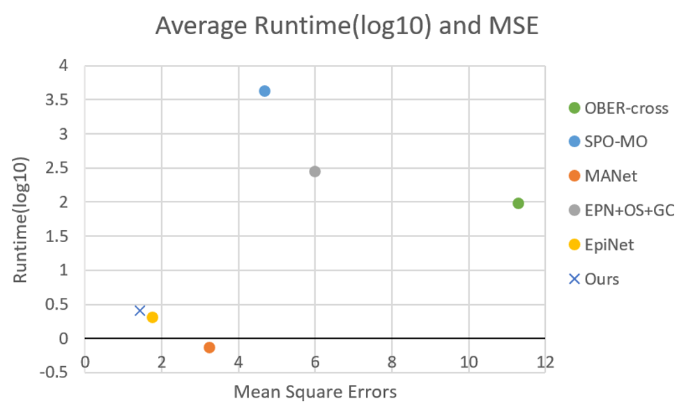
Our research consists of three main parts. Firstly, we enhance the polar plane structure of the light field image. Due to the unique design of light field cameras, EPIs can display directional lines in fixed colors to help visualize light fields. Each line corresponds to a 3D projection and the depth of each point of the scene can be inferred by analyzing the slope of the line. To take advantage of this feature and improve the correlation between views, the horizontal, vertical, and diagonal views are combined to select the input views in data processing, which is similar to the EpiNet. Secondly, we reduce the redundancy between sub-aperture views. Due to the characteristics of the light field image, the baselines between the sub-aperture views are very narrow, and there is a lot of redundancy between the views. As using too many views will increase the amount of computation and negatively affect the predicted results, we use a composite attention module [10] to weigh the feature images after the fusion of each channel, which can not only focus on the most important views but also discover the important areas in the views so that the network can make more effective use of them for depth estimation. Thirdly, we enhance the depth of network training effectively. By integrating the framework of previous deep learning methods, with the network depth reaching a certain level, gradient explosion will occur, resulting in loss failure to converge. In this paper, we use the residual module [11] to overcome the problem of gradient explosion while deepening the network.
The organizational structure of the paper is as follows: Section 2 provides a current research progress research status of light field depth estimation. Section 3 follows with a detailed description of our proposed approach. Simulations and analyses of actual data will be conducted to illustrate the practical value of the method described in Sections 4 and 5. The last section is devoted to the summary of this paper and discussion of future research.
2. Related Work
This paper introduces the depth estimation method of light field from two aspects: methods based on optimization and methods based on deep learning.
2.1 Optimization-based Methods
The depth estimation method of the light field emerged from the depth estimation method of a 2D image, mostly utilizing multi-view matching or refocusing or polar plane image. In terms of multi-view matching, Yu et al. [12] studied geometric relations in baseline space to improve the stereo matching effect of the light field, whereas Heber and Pock [13] used a new PCA matching condition to align sub-aperture images (SAIs). Recently, Chen et al. [14] proposed a depth estimation framework for the regularization of initial label confidence graphs and edge strength weights. Tao et al. [15] used a comparison-based metric to find the optimal parallax for refocusing based on the fact that defocusing diminishes visual sharpness and contrast. Zhou et al. [7] proposed a FocalStackNet, which learned the deep semantic features and local structure information of the light field from focal stack to obtain the depth map. EPIs consist slices of Angle and spatial direction in 2D. Wanner and Goldluecke [16] used a structure tensor to calculate the slope of each line of vertical and horizontal EPIs, changing the study of light field depth into the study of the straight-line slope. Zhang et al. [17] used a rotating parallelogram operator (SPO) to find matching lines from EPIs to solve the depth estimation problem in occluded scenes. Li et al. [18] introduced a new tensor Kullback-Leibler divergence (KLD) to calculate depth by combining EPIs tensors in vertical and horizontal directions. Due to more computing resources are consumed, and the training time becomes longer, however, it is difficult to apply these methods to different data sets.
2.2 Methods Related to Deep Learning
Recently, an increasing number of scholars began to use deep learning methods to obtain the depth of light fields. Shin et al. [8] used a whole network EpiNet, which enhanced the data set and took horizontal, vertical, and diagonal camera views as input. Tsai et al. [19] used channel attention to selectively control input view contribution weights to reduce data redundancy. MANet was proposed by Li et al. [20] as a multi-scale aggregation network with fewer parameters and faster running speed. Li et al. [21] used a lightweight convolutional network LLF-NET that has been trained end-to-end to estimate the light field depth of the wide baseline and also has good performance in the light field of the narrow baseline. These methods improved the prediction results to a large extent, but most of them focus on the number of views selected, ignoring the relationship between views, and a large amount of data redundancy interferes with the accuracy of predicted results. In this paper, we choose a method using compound attention, which effectively combines the relevance between views and completes the depth estimation process efficiently.
3. Proposed Method
In this work, we constructed a compound attention network (CAttNet) for depth estimation from the light field by using compound attention.
A 4D light field is a collection of multi-views, which can be represented by a biplanar parameterization L(x,y,u,v). The connection between the center point and the edge point is described as follows:
(1)
[TeX:] $$L(x, y, u, v)=L\left(x+\left(u^*-u\right) d(x, y), y+\left(v^*-v\right) d(x, y), u^*, v^*\right), u, v \in(1, N),$$where (x,y) is the spatial resolution, (u,v) is the angular resolution. In this paper, we take N=9. [TeX:] $$\left(u^*, v^*\right)$$ represents the coordinates of the central view, which are numbered 40 in the [TeX:] $$N \times N$$ view array (from 00 to 80) specified in this article. d(x,y) represents the parallax between the center view pixel (x,y) and the corresponding pixel of the adjacent view. To estimate the depth of the center view, one must determine the actual offset from the corresponding point in the edge view.
The structure of the CAttNet is shown in Fig. 2. It can be seen that the network consists of three parts: processing layer, weighted layer, and abstraction layer, which will be detailed in following section.

3.1 Processing Layer
According to the study of the depth estimation method of light field, when all views of light field are used as input, more accurate depth estimation results can be obtained to a certain extent, but the calculation speed is more than ten times slower, therefore, we adopt EPI characteristic four-channel input to reduce the amount of data input. Firstly, the horizontal, vertical, and diagonal view streams from the 9×9 view array are stacked and connected, and then sent into the three-layer structure Conv-SeLu-Conv-BN-SeLu block successively. The convolution layer is used to extract image features in this instance. Batch normalization (BN) is used to address data distribution changes in the middle layer during training in order to prevent gradients from vanishing or exploding and to accelerate training. Using the activation function SeLu [22], since it is a regularization scheme based on activation function and has the characteristics of self-normalization. It can converge even with the addition of noise, to reduce the amount of computation, improve the sparsity of the network, reduce the interdependence of parameters, and prevent the disappearance of the gradient. The four branch channels are processed separately, and their parameters are not shared. Then, the outputs of the four branch channels are joined. To adapt to the characteristics of a narrow baseline of the light field, the space kernel size of convolution filters was set to 2×2, the stride was 1, and batch size was 16. The activation function SeLu is calculated as follows:
(2)
[TeX:] $$\operatorname{SeLu}(x)=\lambda_{\text {selu }}\left\{\begin{array}{ll} \alpha_{\text {selu }}\left(e^x-1\right) x \leq 0 \\ x x\gt 0 \end{array},\right.$$where the fixed values of [TeX:] $$\alpha_{\text {selu }} \text { and } \lambda_{\text {selu }}$$ have been calculated to be about 1.6733 and 1.0507.
3.2 Weighted Layer
To obtain depth information, it is important to get effective features from the image, there are a large number of views, and an image of a light field, as mentioned above, the SAIs provide large amounts of information. While also containing a large amount of redundant information, so that our model pays more attention to the training during which views can provide more effective information, as well as an important area in these views. We introduce a compound attention module to weight the feature images, thus reducing the training time and running efficiency of the model. It is composed of a channel attention module and a space attention module, this compound attention module can optimize our method without increasing or decreasing parameters in a stably and reliably manner.
The feature maps from the four branch channels are weighted to determine the significance of "which views." Firstly, the spatial dimension of features extracted by shallow features is compressed to avoid the influence on the channel. This goal can be effectively achieved by maximum pooling and average pooling. The pooled features are then forwarded to a shared network of multilayer perceptron (MLP). Finally, feature vectors are summed and sigmoid functions are used to construct channel attention weights. The attention weight of the channel is calculated as follows:
(3)
[TeX:] $$\begin{aligned} M_c(F)= \sigma(M L P(\operatorname{AvgPool}(F))+\operatorname{MLP}(\operatorname{MaxPool}(F))) \\ =\sigma\left(W_1\left(W_0\left(F_{\text {avg }}^c\right)\right)+W_1\left(W_0\left(F_{\text {max }}^c\right)\right)\right) \end{aligned},$$where [TeX:] $$\sigma(\cdot)$$ represents sigmoid activation function, [TeX:] $$F_{\text {avg }}^c, F_{\max }^c$$ represent average pooling characteristics and maximum pooling characteristics. [TeX:] $$W_0, W_1$$ is the weight of the MLP, [TeX:] $$W_0\in R^{C / r \times C}, W_1 \in R^{C \times C / r} \text {. }$$
Spatial attention selects the key “view regions” using the weighted features obtained by multiplying the channel attention weights and the feature maps connected by our four branch channels. First, maximum pooling and average pooling are performed sequentially. The convolution layer is used to connect and generate a spatial attention diagram after the connection layer. The method for calculating spatial attention weight is:
(4)
[TeX:] $$\begin{aligned} M_S\left(F^{\prime}\right)= \sigma\left(f^{7 \times 7}\left[\operatorname{AvgPool}\left(F^{\prime}\right) ; \operatorname{MaxPool}\left(F^{\prime}\right)\right]\right) \\ =\sigma\left(f^{7 \times 7}\left(\left[{F^{\prime}}_{\text {avg }}^s ; F_{\max }^{\prime}\right]\right)\right) \end{aligned},$$where [TeX:] $$F^{\prime}$$ represents the feature graph weighted by channel attention, [TeX:] $$\sigma(\cdot)$$ represents the sigmoid activation function, and [TeX:] $$f^{7 \times 7}(\cdot)$$ represents the convolution with 7×7 convolution kernel.
As previously noted, the composite attention not only reduces data redundancy but also effectively demonstrates the importance of each view and view region in the parallax estimation step. Because the spatial distance and angle are different, different views or view area the contribution of each is not identical, some repetitive and redundant information of an image of a light field need to give up, let us estimate module can focus on important views and area, access to effective information, to improve the network's overall accuracy and efficiency.
3.3 Abstraction Layer
The level of features in computer vision grows as the network depth increases. Theoretically, deepening the network depth can theoretically achieve better results, but in practical training, the network often exhibits gradient explosion or model degradation, which makes the experimental results worse. To avoid the negative impact produced by network deepening, the residual structure can be used to restore some of the feature information lost due to the previous layer of convolution into the network. To improve the results of the forecast, this paper uses a series of residual models to learn the relationship between features after weighting the feature graph, allowing the network to achieve the same impact when extracting deep features as shallow features. As shown in Fig. 2, a total of four residual modules are used in the extraction layer. Each residual block has two branches, one of which is connects of Conv layer, SeLu layer, and BN layer directly, and the convolution kernel is 2×2 in size for further feature extraction. The other is the residual mapping branch with the structure of the Conv-BN layer, and the size of the convolution kernel is set to 5×5 to ensure that feature graphs have the same size when they are connected. The calculation method of the residual module is as follows:
where x and y represent the input and output respectively. [TeX:] $$W_1 \text { and } W_2$$ represent the two-layer convolution block respectively. [TeX:] $$\sigma(\cdot)$$ stands for ReLU activation function. [TeX:] $$W_s$$ is used to match the dimensional difference between the input and the residual mapping to be learned.
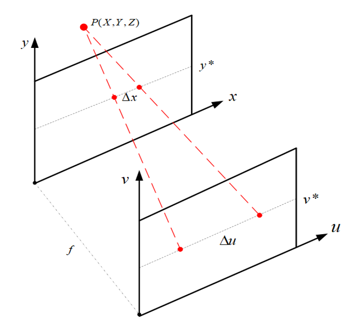
After the residual module, we apply the prediction module using Conv-ReLu-Conv to obtain the final parallax value, with a convolution kernel size of 2×2. According to the geometric relationship between parallax and depth in light field imaging, depth can be quickly calculated to obtain the depth image we need. The relation between the depth of point P in the light field and parallax is shown in Fig. 3. The calculation method of parallax and depth is as follows:
where Z represents the depth value, f represents the fixed focal length of the light field camera, [TeX:] $$\Delta x$$ represents parallax under different viewing angles, and [TeX:] $$\Delta u$$ is the distance between two adjacent light field microlenses.
4. Experiments
4.1 Operation Settings
PyCharm was used as the software environment in the experiment, TensorFlow framework was used as the training backend, Keras library was used to build the network, RMSprop was selected by the optimizer, and batch size was set to 16, the number of network training was set to 600 epochs, 10,000 small batches per epoch. The learning rate for the first 400 epochs was set to [TeX:] $$10^{-4}$$, and then the learning rate for the epochs was reset to [TeX:] $$10^{-5}$$, to improve the accuracy. Mean absolute error (MAE), which has good robustness to outliers, mean square errors (MSE) and bad pixel (BP) are used as the criterion for evaluation of loss.
4.2 Datasets
A 4D Light Field dataset is frequently used as a benchmark for parallax estimation methods for evaluating light field images, which can be compared to a variety of different approaches. It has 24 scenarios divided into four categories: stratified, test, training, and additional. The light field image resolution is 9×9×512×512×3.
4.3 Experimental Contrast
In the training of our model, to judge the error between the model and ground truth, MAE as the evaluation standard can better reflect the situation of the predicted value error. If the MAE value is smaller, the error is considered smaller. MAE is calculated as follows:
To compare the differences between different methods, MSE and BP were selected to evaluate. The accuracy of depth estimation by this method. The smaller the value of the two metrics, the better the algorithm’s performance. MSE and BP are calculated as follows:
where d(x) is the estimated parallax map, gt(x) is ground truth, N is the total number of samples, and t is the threshold of bad pix. We choose the size of 0.07.
In order to further verify the accuracy of our method. Peak signal-to-noise ratio (PSNR) and structural similarity (SSIM) are common image quality evaluation indicators. The higher the value of the two criteria, the better the algorithm's performance. PSNR and SSIM are calculated as follows:
(11)
[TeX:] $$\operatorname{SSIM}(x, y)=\frac{\left(2 \mu_x \mu_y+c_1\right)\left(2 \sigma_{x, y}+c_2\right)}{\left(\mu_x^2+\mu_y^2+c_1\right)\left(\sigma_x^2+\sigma_y^2+c_2\right)},$$where, MAX represents the maximum number of pixels in this image, x and y represent the depth map and ground truth of the scene, respectively. is the mean of the images, [TeX:] $$\sigma_x^2 \text { and } \sigma_y^2$$ are the variances of the images, [TeX:] $$\sigma_{x, y}$$ is the covariance of x and y, and c is a fixed value.
4.4 Experimental Results
We use a 4D Light Field Benchmark dataset to measure the performance of our model. The dataset consists of 28 light field scenarios divided into four subsets: stratified, training, test, and additional. The image resolution is 512×512, and each scene contains 9×9 viewpoints. We use additional 16 light field scenarios to train our proposed network. We use the MSE and BP of light field images to assess the quantitative performance of depth estimation. Qualitative results to show the depth of the light field estimation, we used the eight light field scenes as shown in the images as a comparison—scene from top to bottom is: “turned on,” “dots,” “pyramids,” “stripes,” “boxes,” “cotton,” “dino,” “sideboard.” We were surprised to find that our results had a good effect on the details of the scene objects. Let's zoom in on the feature details as shown in Fig. 4.
Fig. 4.
We compared our model with the following representative models, including OBER-cross [23], SPO-MO [17], MANet [20], EPN+OS+GC [24], and EpiNet [8]. Depth maps obtained from light field images and the corresponding BP diagram is shown in Fig. 5. The green area represents the good pixels, and the red area represents the bad pixels.
Tables 1 and 2 give a quantitative performance comparison of the corresponding MSE (multiplied by 100) and runtime in seconds for each method in different scenarios, and the data with the best performance in the same scenario highlighted in bold. The experimental data show that our method can perform well in most scenarios. Our method compares run time with other algorithms, and the running time is only 0.5 seconds longer than EpiNet after adding modules, indicating that it is excellent practicability.
Fig. 5.
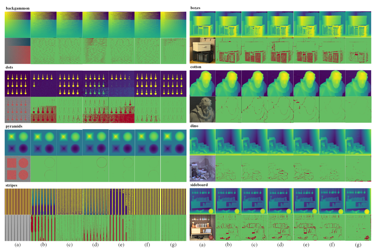
Table 1.
| backgammon | dots | pyramids | stripes | boxes | cotton | dino | sideboard | average | |
|---|---|---|---|---|---|---|---|---|---|
| OBER-cross [23] | 3.504 | 32.524 | 0.301 | 31.717 | 13.129 | 0.939 | 1.952 | 6.284 | 11.294 |
| SPO-MO [17] | 3.450 | 2.781 | 0.050 | 4.118 | 15.494 | 2.161 | 1.968 | 7.515 | 4.692 |
| MANet [20] | 8.573 | 25.915 | 0.445 | 13.975 | 18.398 | 1.689 | 2.710 | 7.513 | 3.244 |
| EPN+OS+GC [24] | 3.699 | 22.369 | 0.018 | 8.731 | 9.314 | 1.406 | 0.565 | 1.744 | 5.981 |
| EpiNet [8] | 3.909 | 1.980 | 0.007 | 0.915 | 6.036 | 0.223 | 0.151 | 0.806 | 1.753 |
| Ours | 4.849 | 0.345 | 0.007 | 0.897 | 4.139 | 0.057 | 0.115 | 1.080 | 1.436 |
The bold font indicates the best performance in each test.
Table 2.
| backgammon | dots | pyramids | stripes | boxes | cotton | dino | sideboard | average | |
|---|---|---|---|---|---|---|---|---|---|
| OBER-cross [23] | 93.940 | 95.790 | 97.200 | 98.050 | 94.240 | 94.290 | 96.350 | 100.230 | 96.261 |
| SPO-MO [17] | 4390.000 | 4381.000 | 4516.000 | 4025.000 | 4368.000 | 4180.000 | 4195.000 | 4226.000 | 4285.125 |
| MANet [20] | 0.730 | 0.730 | 0.730 | 0.730 | 0.730 | 0.730 | 0.730 | 0.730 | 0.730 |
| EPN+OS+GC [24] | 249.234 | 381.063 | 386.781 | 172.297 | 331.375 | 200.031 | 239.734 | 276.313 | 279.604 |
| EpiNet [8] | 2.029 | 2.034 | 2.027 | 2.032 | 2.031 | 2.033 | 2.036 | 2.025 | 2.031 |
| Ours | 2.533 | 2.557 | 2.533 | 2.558 | 2.534 | 2.556 | 2.537 | 2.558 | 2.546 |
The bold font indicates the best performance in each test.
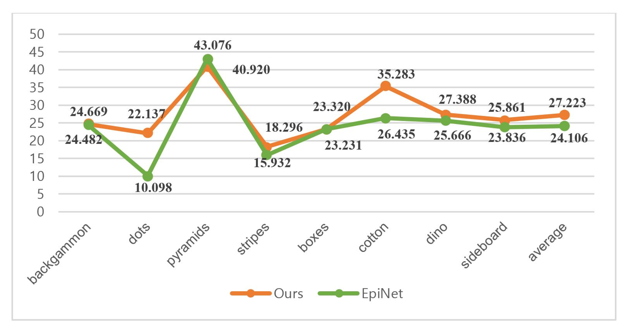
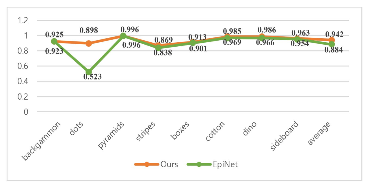
The experimental data show that, both our method and EpiNet perform well in light field scenes. To delve deeper into the accuracy of these two techniques, we use additional image quality evaluation indicators to better reflect the integrity and systematization of the experimental evaluation. The quantitative performance comparison of PSNR and SSIM corresponding to the two methods in different scenarios is shown in Figs. 6 and 7. The green line is EpiNet, whereas the red line represents our technique. It can be concluded that the average performance of our method is better than EpiNet.
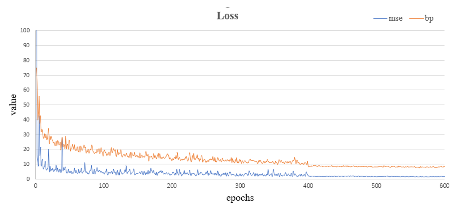
The changes in the BP and MSE indexes on the training set with the number of iterations were observed to investigate the convergence performance of our method on the training data set, and the results are shown in Fig. 8. The red curve represents the MSE index and the blue curve represents the BP index.
5. Ablation Experiments
To demonstrate the reliability of each element in the suggested model architecture, we conducted ablation contrast experiments. The HCI dataset is used to train the suggested network.
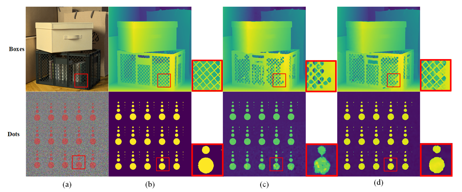
To verify the role of our module in the whole network, we successively added attention block and Resblock, and trained the model for the same amount of times. As a visual comparison, we used the scenario “Origami,” as shown in Fig. 9. Table 3 depicts the performance of our method in the scene following the addition of each module. Measured by the average MSE value, we use “” to indicate adding the module and “” to indicate not adding the module.
Although there are numerous inconsistencies in the background, particularly on certain smooth and continuous planes, the attention module is more effective in paying attention to scene details than Fig. 9 and Table 3. Resblock reduces this error by deepening the network and improving accuracy. The combination of the two can further improve the performance of scene details while reducing errors. This method can better analyze the edge details and Angle information throughout depth estimation process, improve the accuracy of depth map prediction, minimizing the error, and saving time.
Fig. 9.
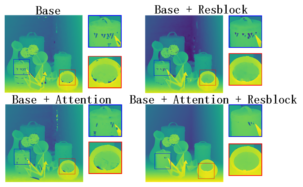
Table 3.
| Attention | Resblock | MSE (average) |
|---|---|---|
| 2.682 | ||
| 2.579 | ||
| 1.977 | ||
| 1.846 |
“” indicates adding the module and “” indicates not adding the module.
6. Conclusion
We propose a new network for depth estimation, by using the light field image geometry and introducing the attention of a complex network, which effectively improves the depth map accuracy of our network. The 4D Light Field Benchmark datasets are used to evaluate the performance of our network and the experimental results show that the CAttNet performs well on the detail place as well as keeping out of the scene, with the hanging time of 18% MSE gain that is substantially less than that of EpiNet. In the future, we intend to continue improving our network so that it can perform better on a smooth background.
Biography

Biography
Biography
Biography
Tao Yan
https://orcid.org/0000-0002-8304-8733
He graduated from Shanghai University in 2010 with a Ph.D. in communication and information systems. He used to work at the School of Information Engineering of Putian University and is now an associate professor. His research interest covers multi-view efficient video coding, bit rate control, and video codec optimization. He is currently in charge of the National Natural Science Foundation of China.
References
- 1 A. C. Tsai, Y . Y . Ou, W. C. Wu, and J. F. Wang, "Occlusion resistant face detection and recognition system," in Proceedings of 2020 8th International Conference on Orange Technology (ICOT), Daegu, South Korea, 2020, pp. 1-4. https://doi.org/10.1109/ICOT51877.2020.9468767doi:[[[10.1109/ICOT51877.2020.9468767]]]
- 2 J. Liu, "Survey of the image recognition based on deep learning network for autonomous driving car," in Proceedings of 2020 5th International Conference on Information Science, Computer Technology and Transportation (ISCTT), Shenyang, China, 2020, pp. 1-6. https://doi.org/10.1109/ISCTT51595.2020.00007doi:[[[10.1109/ISCTT51595.2020.00007]]]
- 3 X. F. Han, H. Laga, and M. Bennamoun, "Image-based 3D object reconstruction: state-of-the-art and trends in the deep learning era," IEEE Transactions on Pattern Analysis and Machine Intelligence, vol. 43, no. 5, pp. 1578-1604, 2021. https://doi.org/10.1109/TPAMI.2019.2954885doi:[[[10.1109/TPAMI.2019.2954885]]]
- 4 H. C. Yang, P . H. Chen, K. W. Chen, C. Y . Lee, and Y . S. Chen, "FADE: feature aggregation for depth estimation with multi-view stereo," IEEE Transactions on Image Processing, vol. 29, pp. 6590-6600, 2020. https://doi.org/10.1109/TIP .2020.2991883doi:[[[10.1109/TIP.2020.2991883]]]
- 5 Y . Zhang, H. Lv, Y . Liu, H. Wang, X. Wang, Q. Huang, X. Xiang, and Q. Dai, "Light-field depth estimation via epipolar plane image analysis and locally linear embedding," IEEE Transactions on Circuits and Systems for Video Technology, vol. 27, no. 4, pp. 739-747, 2017. https://doi.org/10.1109/TCSVT.2016.2555778doi:[[[10.1109/TCSVT.2016.2555778]]]
- 6 A. Ak and P . Le-Callet, "Investigating epipolar plane image representations for objective quality evaluation of light field images," in Proceedings of 2019 8th European Workshop on Visual Information Processing (EUVIP), Roma, Italy, 2019, pp. 135-139. https://doi.org/10.1109/EUVIP47703.2019.8946194doi:[[[10.1109/EUVIP47703.2019.8946194]]]
- 7 W. Zhou, E. Zhou, Y . Yan, L. Lin, and A. Lumsdaine, "Learning depth cues from focal stack for light field depth estimation," in Proceedings of 2019 IEEE International Conference on Image Processing (ICIP), Taipei, Taiwan, 2019, pp. 1074-1078. https://doi.org/10.1109/ICIP .2019.8804270doi:[[[10.1109/ICIP.2019.8804270]]]
- 8 C. Shin, H. G. Jeon, Y . Yoon, I. S. Kweon, and S. J. Kim, "EpiNet: a fully-convolutional neural network using epipolar geometry for depth from light field images," in Proceedings of the IEEE Conference on Computer Vision and Pattern Recognition, Salt Lake City, UT, 2018, pp. 4748-4757. https://doi.org/10.1109/CVPR. 2018.00499doi:[[[10.1109/CVPR.2018.00499]]]
- 9 K. Honauer, O. Johannsen, D. Kondermann, and B. Goldluecke, "A dataset and evaluation methodology for depth estimation on 4D light fields," in Computer Vision–ACCV 2016. Cham, Switzerland: Springer, 2017, pp. 19-34. https://doi.org/10.1007/978-3-319-54187-7_2doi:[[[10.1007/978-3-319-54187-7_2]]]
- 10 S. Woo, J. Park, J. Y . Lee, and I. S. Kweon, "CBAM: convolutional block attention module," in Computer Vision–ECCV 2018. Cham, Switzerland: Springer, 2018, pp. 3-19. https://doi.org/10.1007/978-3-030-012342_1doi:[[[10.1007/978-3-030-012342_1]]]
- 11 K. He, X. Zhang, S. Ren, and J. Sun, "Deep residual learning for image recognition," in Proceedings of the IEEE Conference on Computer Vision and Pattern Recognition, Las V egas, NV , 2016, pp. 770-778. https://doi.org/10.1109/CVPR.2016.90doi:[[[10.1109/CVPR.2016.90]]]
- 12 Z. Y u, X. Guo, H. Lin, A. Lumsdaine, and J. Y u, "Line assisted light field triangulation and stereo matching," in Proceedings of the IEEE International Conference on Computer Vision, Sydney, Australia, 2013, pp. 27922799. https://doi.org/10.1109/ICCV .2013.347doi:[[[10.1109/ICCV.2013.347]]]
- 13 S. Heber and T. Pock, "Shape from light field meets robust PCA," in Computer Vision–ECCV 2014. Cham, Switzerland: Springer, 2014, pp. 751-767. https://doi.org/10.1007/978-3-319-10599-4_48doi:[[[10.1007/978-3-319-10599-4_48]]]
- 14 J. Chen, J. Hou, Y . Ni, and L. P . Chau, "Accurate light field depth estimation with superpixel regularization over partially occluded regions," IEEE Transactions on Image Processing, vol. 27, no. 10, pp. 4889-4900, 2018. https://doi.org/10.1109/TIP .2018.2839524doi:[[[10.1109/TIP.2018.2839524]]]
- 15 M. W. Tao, S. Hadap, J. Malik, and R. Ramamoorthi, "Depth from combining defocus and correspondence using light-field cameras," in Proceedings of the IEEE International Conference on Computer Vision, Sydney, Australia, 2013, pp. 673-680. https://doi.org/10.1109/ICCV .2013.89doi:[[[10.1109/ICCV.2013.89]]]
- 16 S. Wanner and B. Goldluecke, "V ariational light field analysis for disparity estimation and superresolution," IEEE Transactions on Pattern Analysis and Machine Intelligence, vol. 36, no. 3, pp. 606-619, 2014. https://doi.org/10.1109/TPAMI.2013.147doi:[[[10.1109/TPAMI.2013.147]]]
- 17 H. Sheng, P . Zhao, S. Zhang, J. Zhang, and D. Yang, "Occlusion-aware depth estimation for light field using multi-orientation EPIs," Pattern Recognition, vol. 74, pp. 587-599, 2018. https://doi.org/10.1016/j.patcog. 2017.09.010doi:[[[10.1016/j.patcog.2017.09.010]]]
- 18 J. Li and X. Jin, "EPI-neighborhood distribution based light field depth estimation," in Proceedings of 2020 IEEE International Conference on Acoustics, Speech and Signal Processing (ICASSP), Barcelona, Spain, 2020, pp. 2003-2007. https://doi.org/10.1109/ICASSP40776.2020.9053664doi:[[[10.1109/ICASSP40776.2020.9053664]]]
- 19 Y . J. Tsai, Y . L. Liu, M. Ouhyoung, and Y . Y . Chuang, "Attention-based view selection networks for lightfield disparity estimation," Proceedings of the AAAI Conference on Artificial Intelligence, vol. 34, no. 07, pp. 12095-12103, 2020. https://doi.org/10.1609/aaai.v34i07.6888doi:[[[10.1609/aaai.v34i07.6888]]]
- 20 Y . Li, L. Zhang, Q. Wang, and G. Lafruit, "MANet: multi-scale aggregated network for light field depth estimation," in Proceedings of 2020 IEEE International Conference on Acoustics, Speech and Signal Processing (ICASSP), Barcelona, Spain, 2020, pp. 1998-2002. https://doi.org/10.1109/ICASSP40776.2020.9053532doi:[[[10.1109/ICASSP40776.2020.9053532]]]
- 21 Y . Li, Q. Wang, L. Zhang, and G. Lafruit, "A lightweight depth estimation network for wide-baseline light fields," IEEE Transactions on Image Processing, 30, 2288-2300, 2021. https://doi.org/10.1109/TIP.2021. 3051761doi:[[[10.1109/TIP.2021.3051761]]]
- 22 G. Klambauer, T. Unterthiner, A. Mayr, and S. Hochreiter, "Self-normalizing neural networks," Advances in Neural Information Processing Systems, vol. 30, pp. 971-980, 2017.custom:[[[https://arxiv.org/abs/1706.02515]]]
- 23 H. Schilling, M. Diebold, C. Rother, and B. Jahne, "Trust your model: light field depth estimation with inline occlusion handling," in Proceedings of the IEEE Conference on Computer Vision and Pattern Recognition, 2018, pp. 4530-4538. https://doi.org/10.1109/CVPR.2018.00476doi:[[[10.1109/CVPR.2018.00476]]]
- 24 Y . Luo, W. Zhou, J. Fang, L. Liang, H. Zhang, and G. Dai, "EPI-patch based convolutional neural network for depth estimation on 4D light field," in Neural Information Processing. Cham, Switzerland: Springer, 2017, pp. 642-652. https://doi.org/10.1007/978-3-319-70090-8_65doi:[[[10.1007/978-3-319-70090-8_65]]]