Ruiwei Guo
Multi-Dimensional Selection Method of Port Logistics Location Based on Entropy Weight Method
Abstract: In order to effectively relieve the traffic pressure of the city, ensure the smooth flow of freight and promote the development of the logistics industry, the selection of appropriate port logistics location is the basis of giving full play to the port logistics function. In order to better realize the selection of port logistics, this paper adopts the entropy weight method to set up a multi-dimensional evaluation index, and constructs the evaluation model of port logistics location. Then through the actual case, from the environmental dimension and economic competition dimension to make choices and analysis. The results show that port d has the largest logistics competitiveness and the highest relative proximity among the three indicators of hinterland city economic activity, hinterland economic structure, and port operation capacity of different port logistics locations, which has absolute advantages. It is hoped that the research results can provide a reference for the multi-dimensional selection of port logistics site selections.
Keywords: AHP , Entropy Weight Method , Multi-Dimension , Port Logistics Location
1. Introduction
Port logistics is an important node in the overall transport system of cities with shoreline resources. It can not only effectively relieve the pressure of urban traffic, but also ensure the “smooth flow of goods” and promote the development of logistics industry. The appropriate port logistics location selection is conducive to giving full play to the port logistics location function and promoting the economic development of port-related cities and the development of the logistics industry.
At present, several scholars have carried out research on this. Teye et al. [1] used the principle of entropy maximization to construct the location model of port city intermodal transport terminal facilities, so that users could choose to solve the location problem without using multi-user intermodal transport terminals. The model decomposed the research problem into two sub-problems of site selection, analyzed separately, and combined the results for further analysis. The model can reach the conclusion quickly, but the evaluation result of port city intermodal terminal is not objective enough. Komchornrit [2] proposed a new hybrid CFA-MACBETH-PROMETHEE model, which used confirmatory factor analysis to determine load and study the relationship between logistics policy and land port construction geography. The classification evaluation technology is used for measurement, the standard weight is set, and the preference ranking organization method is used to rank the alternative sites. This study can integrate multiple factors for site selection, but the competitiveness analysis of each alternative scheme under this method is subjective and has certain limitations.
To solve the above problems, this paper analyzes the port logistics location selection by combining analytic hierarchy process and entropy weight method, and proposes a multi-dimensional port logistics location selection method based on entropy weight method, which can combine subjective evaluation with objective evaluation to ensure unbiased evaluation results as much as possible [3-5].
2. Material and Methods
2.1 Multi-Dimensional Evaluation Index of Port
In order to evaluate port logistics location selection in a more objective and standardized way, this paper uses multi-dimensional evaluation indices to analyze port logistics location. The evaluation indexes of each dimension selected in this paper are as follows. Before introducing multi-dimensional port evaluation indicators, this paper first analyzes the competitiveness of port logistics areas in Zhejiang Province based on principal component analysis. According to the above evaluation results of port logistics competitiveness of different locations in Zhejiang Province, several different port locations that meet the weight of each indicator are selected from port logistics with better competitiveness evaluation results. Then, each port is selected based on the environmental dimension of the port, and the location of the port is evaluated [6]. Another evaluation dimension of port logistics location in this paper is economic competitiveness. The economic competitiveness of port logistics location is relatively comprehensive, with large package capacity, strong interaction, and strong dynamics [7]. The secondary indicators in the economic competitiveness system of port logistics location include hinterland economic activity level B1, which is the macroscopic performance of port logistics competitiveness; port city economic structure B2 is the port’s goods can be collected and distributed quickly; port operation capability B3 and port infrastructure B4 are effective ways for ports to improve their competitiveness. Materials and carriers are the basis for the normal development of ports [8,9].
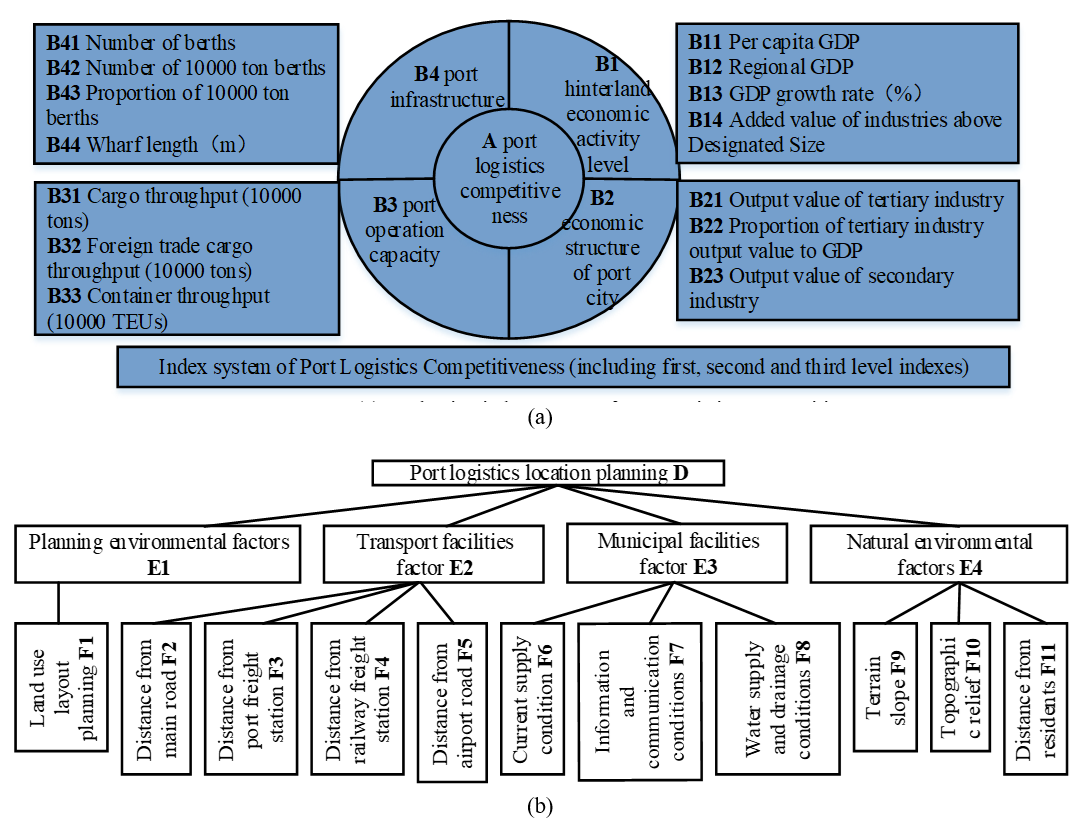
Fig. 1(a) is the evaluation index system of port logistics economic competitiveness, of which there are four secondary evaluation indexes, these have been described in detail above; the third level evaluation indexes have 16, which are GDP per capita (B11), regional GDP (B12), growth rate of regional GDP (B13), industrial added value over designated size (B14, unit: 100 million yuan); tertiary industry output value (B21, unit: 100 million yuan), tertiary industry share of GDP (B22), secondary industry output value (B23, unit: 100 million yuan). Fig. 1(b) is a hierarchical analysis structure diagram of port logistics location selection.
Fig. 1.
2.2 Construction of Evaluation Model
In the previous paper, the multi-dimensional evaluation index of port logistics location selection was constructed, which can be evaluated from two aspects of economic dimension and environmental dimension. Now, based on these selected evaluation indexes, the port logistics location evaluation model is constructed. In the economic dimension of port logistics location, this paper uses entropy weight method to calculate the evaluation indexes, and the evaluation results obtained have the characteristics of strong objectivity, and then uses the analytical hierarchy process to get the evaluation results of strong subjectivity. The two evaluation results obtained are put together for mutual verification to ensure the scientific nature and effectiveness of the weighted results:
(1)
[TeX:] $$\left(x_{i j}\right)_{n \times m}=\left[\begin{array}{cccc} x_{11} & x_{12} & \ldots & x_{1 m} \\ x_{21} & x_{22} & \ldots & x_{2 m} \\ \ldots & \ldots & \ldots & \ldots \\ x_{n 1} & x_{n 2} & \ldots & x_{n m} \end{array}\right]_{n \times m}.$$Formula (1) is the evaluation matrix of entropy weight, where n,m refer to the evaluation index and evaluation item respectively. The evaluation value of the j-th evaluation item under the i-th index is expressed by [TeX:] $$x_{i j}, \text { and } x_{i j} \in[0,1]$$:
(2)
[TeX:] $$p_{i j}=\frac{x_{i j}}{\sum_{j=1}^m x_{i j}} ;(i=1,2, \ldots, n ; j=1,2, \ldots, m) .$$Formula (2) is the formula for calculating the proportion [TeX:] $$p_{i j}$$ of evaluation value of the j-th evaluation project within the scope of the i-th index:
(3)
[TeX:] $$\begin{gathered} E_i=-k \sum_{j=1}^m p_{i j} \ln p_{i j} ; k=\frac{1}{\ln m}\gt 0 \\ \theta_i=\frac{1-e_i}{\sum_{i=1}^n\left(1-e_i\right)}(i=1,2, \ldots, n ; j=1,2, \ldots, m) . \end{gathered}$$Formula (3) is the calculation expression of entropy value [TeX:] $$E_i$$ and entropy weight [TeX:] $$\theta_i$$ of the i-th index, where [TeX:] $$E\left(x_j\right) \in[0,1], \theta_i \in(0,1).$$ When there are N elements in the indicator layer, the pairwise comparison judgment matrix [TeX:] $$F=\left(F_{i j}\right)_{n * n}$$ is obtained, and the important values of element i and element j relative to target E are expressed by [TeX:] $$F_{ij}$$[4]. Formula ([TeX:] $$F X=\lambda_{\max }$$) is the solving equation of eigenvector of judgment matrix [TeX:] $$F=\left(F_{i j}\right)_{n * n},$$ the calculation formula of each index weight can be determined, as shown in formula (4):
(4)
[TeX:] $$w=\left\{\frac{x_1}{\sum_{i=1}^n x_i}, \frac{x_2}{\sum_{i=1}^n x_i}, \ldots, \frac{x_n}{\sum_{i=1}^n x_i}\right\}=\left\{w_1, w_2, \ldots, w_n\right\}.$$The weighting coefficient of the corresponding index obtained by formula (4) should be checked for consistency, C.I., where n refers to the order of the judgment matrix. When C.I.=0, it means that the judgement matrix is in a completely consistent state. If C.I.<0.1, it means that the weighting logic of each index in the indicator layer is reasonable. The consistency ratio test [TeX:] $$C . R .=\frac{C . I .}{R . I .}$$ is used to judge whether the consistency of the matrix is reasonable, where R.I. refers to the average random consistency index [7].
In Fig. 2, the entropy weight should be verified. When there is an index with entropy value [TeX:] $$E\left(x_j\right)=1$$ and entropy weight [TeX:] $$\theta_j=0$$, it means that the index lacks reference value and should be excluded when selecting indicators. When there is an index with entropy value [TeX:] $$E\left(x_j\right)\lt 1$$ and entropy weight [TeX:] $$\theta_j$$ is relatively larger, the index has reference value [10-14]. In view of this, the four reference indicators with small entropy weights (GDP growth rate, growth rate of industries above a certain size, and proportion of secondary and tertiary industries) should be excluded.
Fig. 2.

Table 1 shows the standardized data of GDP per capita, GDP, and value added of industries above designated size for each port after eliminating interference indicators. Combining the actual situation of each port in the port city of H, the above standardized data and entropy weight are processed through the benefit-type formula and the cost-type formula, and a corresponding weighted normalization matrix is constructed:
(5)
[TeX:] $$\left\{\max V_{i j} \mid j \in J_1, i=1,2, \ldots, m\right\} ; V^{-}=\left\{\min V_{i j} \mid j \in J_1, i=1,2, \ldots, m\right\},$$
(6)
[TeX:] $$\left\{\min V_{i j} \mid j \in J_2, i=1,2, \ldots, m\right\} ; V^{-}=\left\{\max V_{i j} \mid j \in J_2, i=1,2, \ldots, m\right\}.$$Formula (5) is a benefit-based formula, where [TeX:] $$J_1$$ refers to the benefit-based index value set, and formula (6) is a cost-based formula, where [TeX:] $$J_2$$ refers to the cost-based index value set.
Table 1.
| Secondary indicators | |||
|---|---|---|---|
| Per capita GDP | GDP (100 million yuan) | Value-added industries | |
| Port a | 0.0462 | 0.0217 | 0.0005 |
| Port b | 0.0948 | 0.1138 | 0.0631 |
| Port c | 0.0451 | 0.0523 | 0.0236 |
| Port d | 0.1214 | 0.2673 | 0.5444 |
| Port e | 0.0546 | 0.0208 | 0.0094 |
| Port f | 0.1366 | 0.1423 | 0.0669 |
| Port g | 0.0744 | 0.0281 | 0.0152 |
| Port h | 0.0514 | 0.025 | 0.0569 |
| Port i | 0.096 | 0.1044 | 0.0619 |
| Port j | 0.1086 | 0.0474 | 0.0232 |
| Port k | 0.1078 | 0.1489 | 0.0729 |
| Port m | 0.0632 | 0.0279 | 0.0617 |
3. Case Analysis
3.1 Evaluation Results of the Environmental Dimension of Port Logistics Location
According to the weight of each index among the environmental factors of the port logistics location—planning environment factor E1, transportation facility factor E2, municipal facilities factor E3, and natural environment factor E4—and checking the consistency, a more suitable port logistics location is selected in the environmental dimension. In terms of environmental dimension, the specific indicators of port logistics location planning are shown in Fig. 3.
Fig. 3.
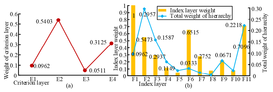
Fig. 3(a) shows that in the criterion level, the transport facilities factor E2 has the largest weight of 0.5403, followed by the port's natural environment factor E4 (0.3125), the planning environment factor E1 (0.0962), and the community facilities factor E3 (0.0511). This is because the port logistics location is the workplace where all-type goods are gathered, distributed, and transshipped. The integrity of transport facilities and the smoothness of transport routes will greatly affect the collection and distribution capacity of port logistics location, so the transport facilities factor occupies the largest weight in the environmental dimension evaluation system. Fig. 3(b) shows that in the index layer of the quasi-lateral layer, the transport facilities factor E2, the distance from the main road F2 is 0.5473. The arterial road runs through the city. The closer it is to the arterial road, the more comprehensive the logistics location function of the port will be and the more restricted the shipping will be. This is why it has the lowest weight in the transport facilities. In the index layer of municipal facilities factor E3, current supply condition F6 accounts for the largest weight of 0.6515. In order to facilitate the handling and loading of goods, the port logistics location is equipped with large-scale logistics-related mechanical equipment, such as conveyors, elevators, etc. In the index layer of E4, the weight of distance from residents F11 is the largest, which is 0.7096.
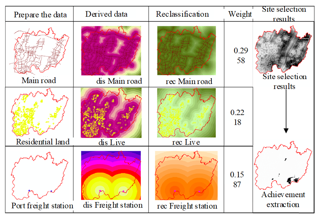
Combining Fig. 3 and Fig. 4, according to the total weight of the level (the index level is relative to the target level), it indicates that in the port logistics location selection, from the environmental dimension, the index weight from the heaviest to the lighter is the distance to the main road F2 (0.2957) > Distance to residents F11 (0.2218) > Distance to port freight station F3 (0.1587) > Land layout planning F1 (0.0962) > Topographic gradient F9 (0.0671) > Distance to railway freight station F4 (0.0621) > Current supply conditions F6 (0.0333) > Distance to airport road F5 (0.0238) > Terrain relief F10 (0.0237) > Information communication condition F7 (0.0141) > Water supply and drainage condition F8 (0.0037). According to the results of port logistics location obtained in Fig. 4, 12 different port logistics locations are selected to rank the economic competitiveness of corresponding logistics locations.
3.2 Evaluation Results of Economic Competition Dimension in Different Location of Port Logistics
In the regional economic competition index system of port logistics, there are three positive ideal solutions [TeX:] $$V^{+}$$ 0.0022, 0.0216, 0.1074 and three negative ideal solutions [TeX:] $$V^{-}$$ 0.0007, 0.0017, 0.0001, respectively for the three third-level indicators of hinterland economic activity level B1. According to formula (6) and formula (7), the economic activity level B1 of the secondary index hinterland and the distance between the positive and negative ideal solutions corresponding to the level B1 can be calculated. The specific results are shown in Fig. 5.
Fig. 5(a) shows the entropy weights of indicators such as GDP per capita (yuan), GDP (100 million yuan), and value added of industries above designated size (100 million yuan) corresponding to each port. It can be seen that the increase of industries above designated size in port logistics location d. The entropy weights such as value (0.1074) and GDP (0.0216) are the highest among the three indicators. In Fig. 5(b), di+ and di- refer to the distance between the measurement index and the positive ideal solution [TeX:] $$V^{+}$$, and the distance between the measurement indicator and the negative ideal solution [TeX:] $$V^{-}$$, respectively. The distance and relative proximity between the exponential and the positive and negative ideal solutions are shown in Fig. 6.
Fig. 5.
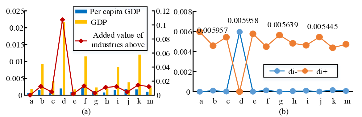
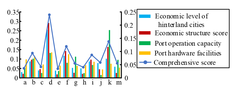
Fig. 6.
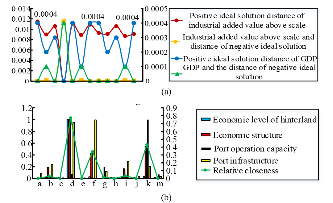
Fig. 6(a) shows that the distance between the GDP per capita index and the positive ideal solution, the distance between the GDP per capita index and the negative ideal solution in each port are both 0; port a has the largest distance from the positive ideal solution (0.0115). Fig. 6(b) shows the degree of approximation of the single-layer index and ideal solution and the corresponding comprehensive ranking. Obviously, port d ranks higher than other ports; From the perspective of port operation capacity in different port logistics locations. After the completion of the consistency check, = 3.0867, C.I. = 0.0433, C.R. =0.0747, and the consistency is good. According to the analysis of analytical hierarchy process, the ranking of logistics competitiveness of 12 ports is port d > k > f > j > b > i > g > h > m > c > e > a.
4. Conclusion
In order to evaluate each port logistics location more comprehensively, this paper proposes a multi-dimensional port logistics location selection method based on the entropy weight method, which evaluates each port logistics location from multiple dimensions and different indicators. The evaluation scores of various indicators of different port logistics locations are different. In order to select port logistics locations that are in an excellent position in various dimensions, this study uses two methods, entropy weight method and analytic hierarchy process. The research results show that from the relevant evaluation results of the economic activities of hinterland cities, it can be seen that the logistics compe¬titiveness of port d logistics location is the largest, with a relative closeness of 1, occupying an absolute dominant position. Judging from the corresponding evaluation results of port operation capability, port d has the greatest competitive advantage. From the perspective of port infrastructure, port f occupies an absolute dominant position. Judging from the evaluation results of the port’s comprehensive logistics location competitiveness, port d has the strongest comprehensive competitive advantage. The method studied in this paper has achieved certain results, achieved the design purpose of this method, and realized the multi-dimensional selection of port logistics location. However, the method in this paper still has some shortcomings, which need to be improved in the follow-up research in order to achieve a wider range of practical application.
Biography
Ruiwei Guo
https://orcid.org/0000-0003-0023-4563
He received was born in March 1986, male, senior experimentalist. He graduated in July of 2010 from Zhejiang Normal University with a bachelor’s degree of Trans-portation and graduated in March of 2017 from Hangzhou Dianzi University with a master’s degree of Logistics Engineering. He now works in Taizhou Vocational College of Science and Technology as a teacher in Logistics Major. His main research in logistics engineering, supply chain management, agricultural economics, vocational education, etc. He has published 8 academic articles, presided over one provincial project and 6 municipal project, participated in more than 10 horizontal and vertical projects of different levels, and won 1 provincial prize and 1 municipal prize in scientific research achievements.
References
- 1 C. Teye, M. G. Bell, and M. C. Bliemer, "Entropy maximising facility location model for port city intermodal terminals," Transportation Research Part E: Logistics and Transportation Review, vol. 100, pp. 1-16, 2017. https://doi.org/10.1016/j.tre.2017.01.006doi:[[[10.1016/j.tre.2017.01.006]]]
- 2 K. Komchornrit, "The selection of dry port location by a hybrid CFA-MACBETH-PROMETHEE method: a case study of Southern Thailand," The Asian Journal of Shipping and Logistics, vol. 33, no. 3, pp. 141-153, 2017. https://doi.org/10.1016/j.ajsl.2017.09.004doi:[[[10.1016/j.ajsl.2017.09.004]]]
- 3 Y . Tian, "Impact of Ningbo port logistics on regional economic development of Zhejiang Province," Asian Agricultural Research, vol. 11, no. 7, pp. 16-18, 2019.custom:[[[https://ideas.repec.org/a/ags/asagre/299721.html]]]
- 4 H. Wei and M. Dong, "Import-export freight organization and optimization in the dry-port-based cross-border logistics network under the Belt and Road Initiative," Computers & Industrial Engineering, vol. 130, pp. 472-484, 2019. https://doi.org/10.1016/j.cie.2019.03.007doi:[[[10.1016/j.cie.2019.03.007]]]
- 5 H. Wei and Z. Sheng, "Dry ports-seaports sustainable logistics network optimization: considering the environment constraints and the concession cooperation relationships," Polish Maritime Research, vol. 24, no. s3, pp. 143-151, 2017. https://doi.org/10.1515/pomr-2017-0117doi:[[[10.1515/pomr-2017-0117]]]
- 6 E. Irannezhad, C. G. Prato, and M. Hickman, "An intelligent decision support system prototype for hinterland port logistics," Decision Support Systems, vol. 130, article no. 113227, 2020. https://doi.org/10.1016/j.dss. 2019.113227doi:[[[10.1016/j.dss.2019.113227]]]
- 7 G. Lyu, L. Chen, and B. Huo, "The impact of logistics platforms and location on logistics resource integration and operational performance," The International Journal of Logistics Management, vol. 30, no. 2, pp. 549568, 2019. https://doi.org/10.1108/IJLM-02-2018-0048doi:[[[10.1108/IJLM-02-2018-0048]]]
- 8 T. Hamid, D. Al-Jumeily, and J. Mustafina, "Evaluation of the dynamic cybersecurity risk using the entropy weight method," in Technology for Smart Futures. Cham, Switzerland: Springer, 2018, pp. 271-287. https://doi.org/10.1007/978-3-319-60137-3_13doi:[[[10.1007/978-3-319-60137-3_13]]]
- 9 F. Liu, S. Zhao, M. Weng, and Y . Liu, "Fire risk assessment for large-scale commercial buildings based on structure entropy weight method," Safety Science, vol. 94, pp. 26-40, 2017. https://doi.org/10.1016/j.ssci. 2016.12.009doi:[[[10.1016/j.ssci.2016.12.009]]]
- 10 M. H. Ha, Z. Yang, and J. S. L. Lam, "Port performance in container transport logistics: a multi-stakeholder perspective," Transport Policy, vol. 73, pp. 25-40, 2019. https://doi.org/10.1016/j.tranpol.2018.09.021doi:[[[10.1016/j.tranpol.2018.09.021]]]
- 11 T. Li and W. Yang, "Solution to chance constrained programming problem in swap trailer transport organisation based on improved simulated annealing algorithm," Applied Mathematics and Nonlinear Sciences, vol. 5, no. 1, pp. 47-54, 2020. https://doi.org/10.2478/amns.2020.1.00005doi:[[[10.2478/amns.2020.1.00005]]]
- 12 H. G. Citil, "Important notes for a fuzzy boundary value problem," Applied Mathematics and Nonlinear Sciences, vol. 4, no. 2, pp. 305-314, 2019. https://doi.org/10.2478/AMNS.2019.2.00027doi:[[[10.2478/AMNS.2019.2.00027]]]
- 13 B. Cao, J. Zhao, Y . Gu, Y . Ling, and X. Ma, "Applying graph-based differential grouping for multiobjective large-scale optimization," Swarm and Evolutionary Computation, vol. 53, article no. 100626, 2020. https://doi.org/10.1016/j.swevo.2019.100626doi:[[[10.1016/j.swevo.2019.100626]]]
- 14 B. Zeng, J. Feng, N. Liu, and Y . Liu, "Co-optimized public parking lot allocation and incentive design for efficient PEV integration considering decision-dependent uncertainties," IEEE Transactions on Industrial Informatics, vol. 17, no. 3, pp. 1863-1872, 2021. https://doi.org/10.1109/TII.2020.2993815doi:[[[10.1109/TII.2020.2993815]]]
- 15 J. Lee, J. G. Andrews, and D. Hong, "Spectrum-sharing transmission capacity," IEEE Transactions on Wireless Communications, vol. 10, no. 9, pp. 3053-3063, 2011. https://doi.org/10.1109/TWC.2011.070511. 101941doi:[[[10.1109/TWC.2011.070511.10]]]