Zhang Yong , Guoteng Hui and Lei Zhang
Multi-Description Image Compression Coding Algorithm Based on Depth Learning
Abstract: Aiming at the poor compression quality of traditional image compression coding (ICC) algorithm, a multi-description ICC algorithm based on depth learning is put forward in this study. In this study, first an image compression algorithm was designed based on multi-description coding theory. Image compression samples were collected, and the measurement matrix was calculated. Then, it processed the multi-description ICC sample set by using the convolutional self-coding neural system in depth learning. Compressing the wavelet coefficients after coding and synthesizing the multi-description image band sparse matrix obtained the multi-description ICC sequence. Averaging the multi-description image coding data in accordance with the effective single point’s position could finally realize the compression coding of multi-description images. According to experimental results, the designed algorithm consumes less time for image compression, and exhibits better image compression quality and better image reconstruction effect.
Keywords: Compressed Sensing , Deep Learning , ICC Algorithm , Multi-Description Image Coding
1. Introduction
In the traditional image processing, the image can obtain as much sampling data as possible through sampling, and discard less important data during the storage or transmission. This processing mode reduces the data processing efficiency, and the compressed data accounts for a small proportion, resulting in a large waste of resources [1]. Therefore, new ways should be taken to improve the image processing effect. At present, the classical imaging mode faces the problems of increased data volume, high storage and signal processing cost in involving ultra-wideband communication and digital images [2]. Therefore, it is necessary to study large-scale and high-dimensional image processing. Owe to increased efficiency in image storage and transmission, image compression coding (ICC) technology has attracted extensive attention. Generally speaking, ICC technology converts a large data file into a smaller one of the same nature by the virtue of inherent redundancy and correlation of image data, so that data can be stored and transmitted more efficiently [3].
Many countries have conducted in-depth researches on this technology. In [4], the authors put forward an ICC method using orthogonal sparse coding and texture feature extraction to represent image blocks. This method improves the quality of image reconstruction and reduces the decoding time by using the gray level orthogonal sparse transformation. It also measures the variation coefficient characteristics between the range and the domain block by using the correlation coefficient matrix, thus reducing the redundancy and encoding time. In [5], a fast fractal ICC (FICC) method based on square weighted centroid feature (SWCF) is put forward. FICC reduces the redundancy of image data based on the similarity of image by using compression affine transformation, thus achieving image data compression, with the characteristics of high compression ratio and simple recovery. However, FICC is also limited due to complex coding. To this end, a fast FICC algorithm based on SWCF is put forward.
Based on the research mentioned above, a multi-description ICC algorithm on the basis of depth learning is proposed. In this study, it first designs the image compression algorithm based on multi-description coding technology, and then optimizes the algorithm based on depth learning method, achieving better image processing quality.
2. Image Compression Sample Collection based on Compressed Sensing Theory
Multi-description coding is a method put forward in recent years for real-time signal transmission in unreliable networks. The common problem of the existing multi-description coding methods is that the reconstruction quality as well as the ability to resist error and packet loss depend on the number of descriptions, and the more descriptions, the higher the computational complexity and the lower the coding efficiency. Compressed sensing technology uses a small number of observations to extract the effective information in the signal. The amount of information is evenly distributed among the observations. Each observation can be regarded as a description of the original signal, and the image is divided into blocks to form multi-descriptions. The code stream realizes the collection of image compression samples.
2.1 Multi-Description Image Compression Algorithms
Multi-description ICC is on the basis of iterative function system and the collage theorem, which can achieve image compression by using the self-similarity between images [6]. To obtain M descriptions of an image, the source should be divided into M subsets. It takes a 512×512 grayscale image as an example to obtain two descriptions. Units are divided into 64×64 blocks, and 1, 2 are cross-labeled to form two subsets (1 for subset 1; 2 for subset 2), and then two descriptions are generated according to the following steps:
Description 1: Quantize subset 1 with a smaller perceptual quantization step size. Predict subset 2 with the subset 1 after reconstruction. Quantize the prediction redundancy with a larger fixed quantization step size.
Description 2: Quantize subset 2 with a smaller perceptual quantization step size. Predict subset 1 with the subset 2 after reconstruction. Quantize the prediction redundancy with a larger fixed quantization step size.
The image block is identified based on the local features of the image, and [TeX:] $$d_i$$ denotes the variance of the image block, see formula (1).
In formula (2), [TeX:] $$$$ denotes the size of the video image block; [TeX:] $$\bar{p}_i$$ denotes the gray value; [TeX:] $$p_{i j}$$ denotes the gray value of the [TeX:] $$i$$-th block and the [TeX:] $$j$$-th pixel.
[TeX:] $$\bar{d}$$ denotes the image block’s average variance, and the formula (3) can be seen as follows.
In formula (3), [TeX:] $$d_{\min }=\min \left\{d_1, d_2, \ldots, d_n\right\}$$ denotes the smallest variance; [TeX:] $$d_{\max }=\max \left\{d_1, d_2, \ldots, d_n\right\}$$ denotes the largest variance.
According to the variance mean, the classification criterion of image block [TeX:] $$x_i$$ is expressed as formula (4).
(4)
[TeX:] $$x_i \in\left\{\begin{array}{cc} P & \bar{d}_i \leq T_1 \\ B & T_1<\bar{d}_i \leq T_2 \\ W & \bar{d}_i>T_2 \end{array}\right.$$In formula (4), [TeX:] $$T_1$$ and [TeX:] $$T_2$$ represent the classification threshold. [TeX:] $$P$$ represents smooth and fast, [TeX:] $$B$$ denotes edge blocks, and [TeX:] $$W$$ represents texture blocks.
3. Multi-Description ICC Algorithm based on Deep Learning
In the multi-description image compression algorithm, seeking the best matching image block for each image block is not rapid enough, and the result of coding implementation is not satisfactory, so some algorithms should be taken to optimize the process.
3.1 Processing Multi-Description ICC Sample Set based on Deep Learning
The coefficient of variation is the ratio of the standard deviation of the data to the average value, which reflects the degree of dispersion between the data and is affected by the variance and the average value. Therefore, this paper extracted the coefficient of variation of the image block as a new feature. Fitting the coefficient of variation to the coefficient of polynomial can effectively reduce the difficulty of searching. This paper dealt with the character set of multi-description ICC samples, and used coefficients to code samples. First, it used the difference between the single point sub-band and the coefficient amplitude to distinguish the initial node value of the low and high frequency sub-band [7], and calculate the single point number of the low frequency sub-band according to the initial node value of 1. The high-frequency sub-band set of the root node was set to 2, and the coordinate sets of the low and high frequency sub-band were set to 3 and 4, respectively. Then the root node of these two sets of coordinate sets can be expressed as formula (5).
(5)
[TeX:] $$P_4(T(i, j ; \text { type }))=\left\{\begin{array}{l} T(i, j ; A):(i, j) \in O(i, j), \quad \text { type }=A \\ T(i, j ; B) \cup(i, j):(i, j) \in O(i, j), \quad \text { type }=B \end{array}\right.$$It is known that there is a certain correlation between the coordinate root nodes. Through the wavelet domain image data, the original low frequency sub-band set of the high frequency components are used to count the characteristics of different wavelet domain image data components [8]. The high-frequency components of the coefficient coding samples are determined using the reconnaissance output images of different imaging mechanisms, and the correlation coefficient amplitude based on the data of the high-frequency components are established [9]. The amplitude coding calculation is as formula (6).
The wave domain of the image is determined according to the amplitude coding and the dynamic range of the coefficient amplitude, and the threshold sequence of the encoded amplitude coefficient is determined by the concentration of the image bit depth, as shown in formula (7).
where [TeX:] $$T_n=2^n$$ and [TeX:] $$n$$ are the indices when the values are actually encoded, and the difference between the thresholds constituted by the set elements can be set to 2. The coded character classification calculation of coefficient amplitude division is as formula (8).
where [TeX:] $$c_{i j}$$ is the coordinate element of coefficient coding. It is known that the average number of amplitudes of multi-description ICC is [TeX:] $$\left\lceil\log _2 T_{n+1}\right\rceil=(n+1)$$, then the number of added bits needs to be equal to the average number of amplitudes, and the number of bits of the coefficient amplitude is calculated where [TeX:] $$\lambda$$ represents the set of coordinate elements in formula (9).
(9)
[TeX:] $$\sigma=\sum_{n=0}^n \lambda\left\lceil\log _2 T_{n+1}\right\rceil=\sum_{n=0}^n(n+1) \lambda$$where the encoding of the wave domain image data is equivalent to the number of bits. The number of bits is required in determination of the coefficient amplitude of the deep learning multi-description image compression encoding sample. The corresponding coordinate position needs to be determined so as to determine the encoding coefficient on the basis of retaining the original data. The output code stream of the coefficient coding samples is determined based on coefficient values [10] according to formula (10).
Bring the binary values [TeX:] $$r$$ and [TeX:] $$l$$ into the code stream can find the elements of the output coding samples. The detection operator and the set division operator are determined according to the normalization operator, and the detection operator of the non-empty subset [TeX:] $$S$$ is calculated according to formula (11).
When there is a significant single point relative to the threshold of [TeX:] $$T=2^n$$, for some character set statistics in the coordinate set satisfying [TeX:] $$\zeta(s)=1$$, the divided character set has an intersection in the non-empty multivariate coordinate. Therefore, to separate the non-empty individual subsets from it, the expression of the deep learning multi-description ICC sample character set is determined as formula (12).
where[TeX:] $$S_1, S_2, \cdots, S_d$$ are the sample characters in the non-empty subset [TeX:] $$s$$ of the detection operator. By processing the deep learning multi-description ICC sample character set, the characters in the sample character set are converted into coded data, and the frequency band coefficient matrix is synthesized using coded data.
3.2 Synthesizing Multi-Description Image Band Sparse Matrix
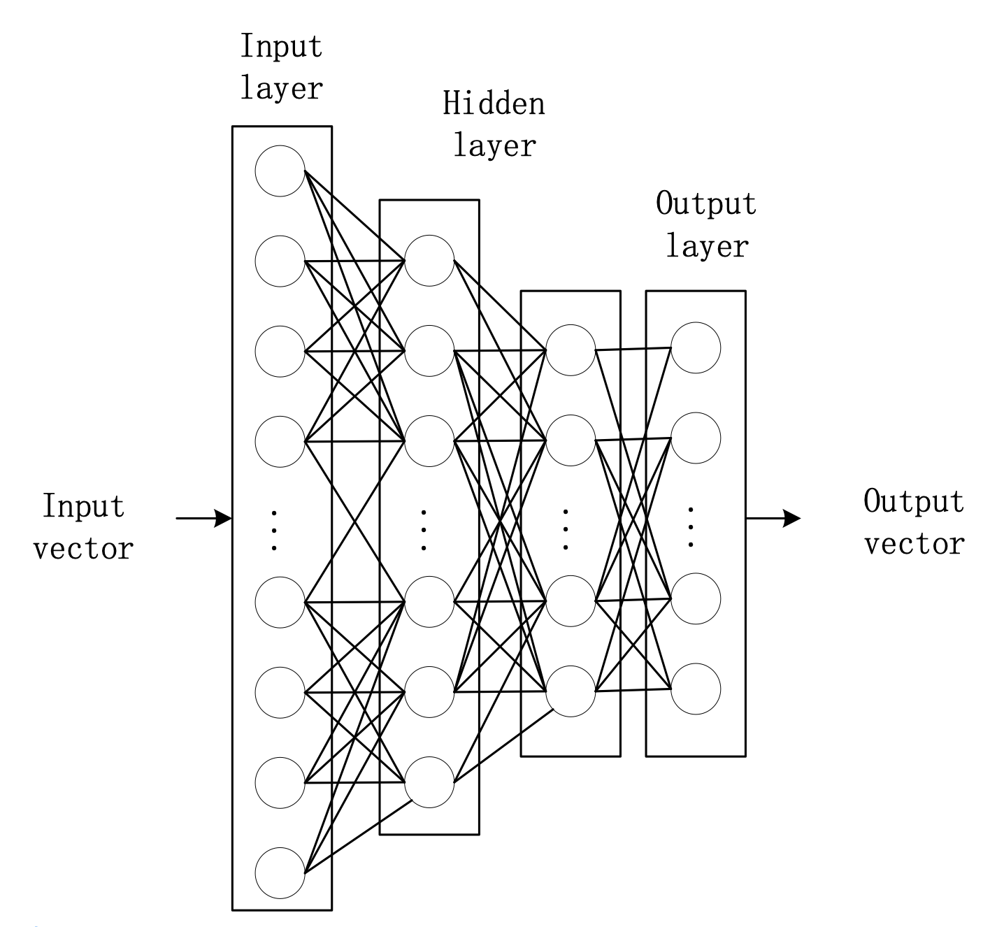
The convolutional sparse self-coding neural network model is applied to compress the coded sample data of multi-description images, and the encoded wavelet coefficients are compressed. Fig. 1 shows the model structure.
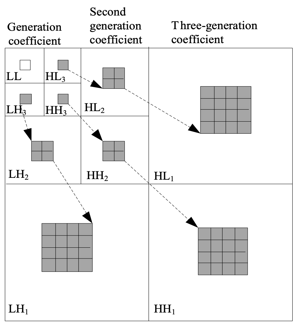
It arranges the coefficients after compression and transform, and organizes the coefficients into a zero-number structure [11]. The convolutional sparse self-coding neural network model is used to iteratively rearrange the band coefficient grades, and each transformation coefficient corresponds to the corresponding point (Fig. 2).
4. Experimental Analysis
The feasibility of the proposed algorithm and the methods proposed in [4] and [5] were comparatively analyzed by selecting 100 pictures in the network as the test set.
Fig. 3.
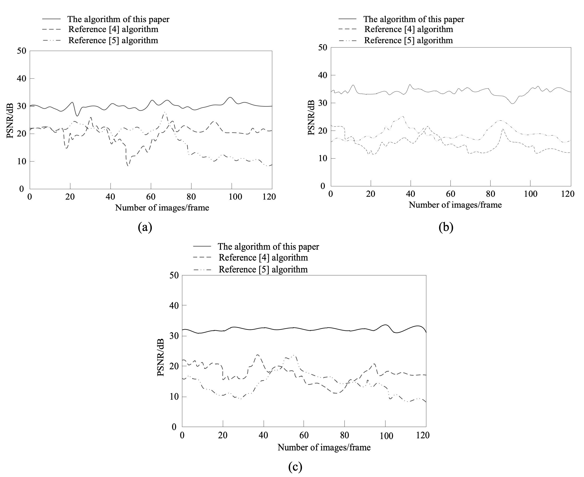
4.1 Multi-Description Image Compression Quality at Different Compression Ratios
The proposed algorithm and the algorithms in [4] and [5] were adopted to perform multi-description image compression. Its quality of the above algorithms under different compression ratios were tested by taking peak signal-to-noise ratio (PSNR) as evaluation index.
Fig. 3 shows that the PSNR of the proposed algorithm slightly fluctuated at about 30 dB, which was basically stable. However, the PSNR of the methods in [4] and [5] was lower than 30 dB. When the compression ratio was 32, 64, and 128, the PSNR of other two methods was still far lower than that of the proposed algorithm. This proves that the proposed algorithm can well compress multi-description images under different compression ratios.
4.2 Image Reconstruction Quality
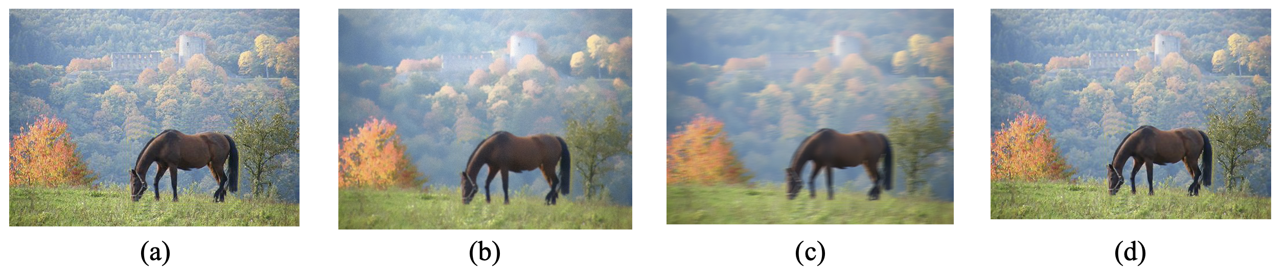
The image reconstruction effects of the three methods when compressing and coding multi-description images were comparatively analyzed, as shown in Fig. 4.
5. Conclusion
In this study, a multi-description ICC algorithm based on compressed sensing and deep learning was put forward. The proposed algorithm used compressed sensing to obtain multi-description image features, and realized multi-description ICC through deep learning. According to experimental results, the algorithm can well realize image compression and reconstruction, with excellent compression coding quality, so it has a great application prospect.Biography
Yong Zhang
https://orcid.org/0000-0003-2828-4220
He received B.S. degree in mathematical Science from Qufu Normal University in 2013, and M.A.Sc. degree in traffic information engineering and control discipline from Civil Aviation Flight University of China in 2016. He is currently an engineer in the School of Computer Science, Civil Aviation Flight University of China, Guanghan, Sichuan. His research interests include computer vision, artificial intelligences.
Biography
Guoteng Hui
https://orcid.org/0000-0003-1283-2827
He received B.Eng. degree in transportation discipline from Binzhou University in 2015, and M.A.Sc degree in traffic information engineering and control discipline from Civil Aviation Flight University of China in 2018. He is currently an engineer in the School of Computer Science, Civil Aviation Flight University of China, Guanghan, Sichuan. His research interests include computer vision, embedded development, and UAVs.
Biography
Lei Zhang
https://orcid.org/0000-0003-1362-9468
He received B.S degree in software engineering from Xi'an University of Posts and Telecommunications in 2016, M.S. degree in transportation engineering from Civil Aviation Flight University of China in 2019. He is currently an engineer in the information center of Civil Aviation Flight University of China. His research interests include network information security and smart campus.
References
- 1 P . Li and K. T. Lo, "Survey on JPEG compatible joint image compression and encryption algorithms," IET Signal Processing, vol. 14, no. 8, pp. 475-488, 2020.doi:[[[10.1049/iet-spr.2019.0276]]]
- 2 H. Y u and L. Y . Hu, "Fractal image texture detail enhancement based on Newton iteration algorithm," Computer Simulation, vol. 38, no. 2, pp. 263-266, 2021.custom:[[[-]]]
- 3 R. Gupta, D. Mehrotra, and R. K. Tyagi, "Computational complexity of fractal image compression algorithm," IET Image Processing, vol. 14, no. 17, pp. 4425-4434, 2020.doi:[[[10.1049/iet-ipr.2019.0489]]]
- 4 H. Pang and A. Zhang, "Sparse coding algorithm for fractal image compression based on coefficient of variation," Application Research of Computers, vol. 38, no. 8, pp. 2485-2489, 2021.custom:[[[-]]]
- 5 L. Wang and Z. Liu, "Fast fractal image compression coding based on square weighted centroid feature," Telecommunication Engineering, vol. 60, no. 8, pp. 871-875, 2020.custom:[[[-]]]
- 6 T. Tian, H. Wang, L. Zuo, C. C. J. Kuo, and S. Kwong, "Just noticeable difference level prediction for perceptual image compression," IEEE Transactions on Broadcasting, vol. 66, no. 3, pp. 690-700, 2020.doi:[[[10.1109/tbc.2020.2977542]]]
- 7 W. Zhang, S. Zou, and Y . Liu, "Iterative soft decoding of Reed-Solomon codes based on deep learning," IEEE Communications Letters, vol. 24, no. 9, pp. 1991-1994, 2020.doi:[[[10.1109/lcomm.2020.2992488]]]
- 8 M. W. Li, D. Y . Xu, J. Geng, and W. C. Hong, "A ship motion forecasting approach based on empirical mode decomposition method hybrid deep learning network and quantum butterfly optimization algorithm," Nonlinear Dynamics, vol. 107, no. 3, pp. 2447-2467, 2022.doi:[[[10.1007/s11071-021-07139-y]]]
- 9 J. S. Wekesa, J. Meng, and Y . Luan, "Multi-feature fusion for deep learning to predict plant lncRNA-protein interaction," Genomics, vol. 112, no. 5, pp. 2928-2936, 2020.doi:[[[10.1016/j.ygeno.2020.05.005]]]
- 10 V . Monga, Y . Li, and Y . C. Eldar, "Algorithm unrolling: interpretable, efficient deep learning for signal and image processing," IEEE Signal Processing Magazine, vol. 38, no. 2, pp. 18-44, 2021.doi:[[[10.1109/msp.2020.3016905]]]
- 11 E. Balevi and J. G. Andrews, "Autoencoder-based error correction coding for one-bit quantization," IEEE Transactions on Communications, vol. 68, no. 6, pp. 3440-3451, 2020.doi:[[[10.1109/tcomm.2020.2977280]]]